Backtesting from Scratch & with VectorBT
Build a vectorised backtest by hand, then reproduce it with VectorBT and realistic costs.
- ·Positions from signals
- ·Returns & equity curve
- ·Costs & slippage
- ·VectorBT from_signals
- ·Reading pf.stats()
- ·Long-only vs both
You now have a strategy idea and you can place orders. The dangerous temptation at this point is to just switch it on and hope. Don't. The single most valuable thing code gives a trader is the ability to ask, "what would this rule have done over the last year?" - and get an honest answer in seconds. That's backtesting, and it's the difference between a hunch and an edge.
A backtest replays your strategy over historical data: it generates signals, pretends to trade on them, and tracks what your account would have done. In this chapter we'll build one by hand first - slowly, one column at a time - so you understand exactly what's happening and never treat a backtest as a black box. Then we'll reproduce the very same result with VectorBT, a fast, battle-tested backtesting library, and add the realistic costs that turn a fantasy result into a believable one.
Our example strategy throughout is the classic EMA crossover: when a fast moving average rises above a slow one, the trend is up, so be long; when it crosses back below, get out. Simple, but the perfect vehicle for learning the mechanics.
Part 1 - A backtest by hand
From indicator to signal
The first step is turning an indicator into a yes/no decision. We compute a fast EMA (10-day) and a slow EMA (30-day), and our signal is simply 1 when fast is above slow (be long) and 0 otherwise (be flat). An EMA - exponential moving average - is just a smoothed average that weights recent prices more heavily; we met it back in the indicators chapters.
# Step 1 of a by-hand backtest: turn an EMA crossover into BUY/SELL signals.
import datetime
import os

from openalgo import api, ta

client = api(
    api_key=os.getenv("OPENALGO_API_KEY", "your_api_key_here"),
    host=os.getenv("OPENALGO_HOST", "http://127.0.0.1:5000"),
)

end = datetime.date.today()
start = end - datetime.timedelta(days=400)
df = client.history(symbol="SBIN", exchange="NSE", interval="D",
                    start_date=str(start), end_date=str(end))
close = df["close"].astype(float)

# A trend signal: fast EMA above slow EMA = uptrend (be long), below = flat.
fast = ta.ema(close, 10)
slow = ta.ema(close, 30)
signal = (fast > slow).astype(int)   # 1 when bullish, 0 otherwise

print(f"Bars: {len(close)}")
print(f"Days the signal says 'be long': {int(signal.sum())}")
print(signal.tail(5).to_string())Bars: 273 Days the signal says 'be long': 188 timestamp 2026-06-17 1 2026-06-18 1 2026-06-19 1 2026-06-22 1 2026-06-23 1
The most important line: .shift(1)
Here is the rule that separates an honest backtest from a fantasy. You only know today's signal after today's candle closes. So you cannot trade on it today - the earliest you can act is the next bar. We express that one-bar delay with .shift(1), which slides the signal forward one day to become the position you actually hold.
Skip this and you commit look-ahead bias: your backtest "buys" using information it couldn't have had yet, producing gorgeous results that evaporate in live trading. This is the number-one way beginners fool themselves.
# Step 2: the .shift(1) that stops you from cheating (trading on today's close).
import datetime
import os

from openalgo import api, ta

client = api(
    api_key=os.getenv("OPENALGO_API_KEY", "your_api_key_here"),
    host=os.getenv("OPENALGO_HOST", "http://127.0.0.1:5000"),
)

end = datetime.date.today()
start = end - datetime.timedelta(days=400)
df = client.history(symbol="SBIN", exchange="NSE", interval="D",
                    start_date=str(start), end_date=str(end))
close = df["close"].astype(float)
signal = (ta.ema(close, 10) > ta.ema(close, 30)).astype(int)

# You only SEE today's signal after today's close, so you can only act on it
# TOMORROW. shift(1) moves the signal forward one bar = the position you hold.
position = signal.shift(1).fillna(0)

print("Signal today vs position held (note the one-day lag):")
preview = close.to_frame("close")
preview["signal"] = signal
preview["position"] = position
print(preview.tail(6).to_string())
print("\nWithout shift(1) you would be 'buying the close you already saw' "
"- a classic look-ahead bug that fakes great results.")Signal today vs position held (note the one-day lag):
close signal position
timestamp
2026-06-16 1015.30 0 0.0
2026-06-17 1026.50 1 0.0
2026-06-18 1042.70 1 1.0
2026-06-19 1035.10 1 1.0
2026-06-22 1040.75 1 1.0
2026-06-23 1023.60 1 1.0
Without shift(1) you would be 'buying the close you already saw' - a classic look-ahead bug that fakes great results.Look-ahead bias is the cardinal sin of backtesting. Any time your position on a given day depends on data from that same day or later, your results are fiction. .shift(1) on your signal is the simplest cure - make it a reflex.
Strategy returns
Now the payoff. The market's daily return is just close.pct_change(). Your strategy return is the market's return only on the days you held a position - that's position * market_return. On days you were flat, your return is zero: cash earns nothing, but it also can't lose. This single multiplication is the heart of every vectorised backtest.
# Step 3: strategy return = market return ONLY on days you held a position.
import datetime
import os

from openalgo import api, ta

client = api(
    api_key=os.getenv("OPENALGO_API_KEY", "your_api_key_here"),
    host=os.getenv("OPENALGO_HOST", "http://127.0.0.1:5000"),
)

end = datetime.date.today()
start = end - datetime.timedelta(days=400)
df = client.history(symbol="SBIN", exchange="NSE", interval="D",
                    start_date=str(start), end_date=str(end))
close = df["close"].astype(float)
position = (ta.ema(close, 10) > ta.ema(close, 30)).astype(int).shift(1).fillna(0)

# Daily % change of the stock.
market_ret = close.pct_change().fillna(0)
# You earn the day's move only when position == 1 (you were long).
strategy_ret = position * market_ret

print(f"Average daily market return  : {market_ret.mean() * 100:.3f}%")
print(f"Average daily strategy return: {strategy_ret.mean() * 100:.3f}%")
print(f"Days in the market: {int((position == 1).sum())} of {len(position)}")
print("On flat days the strategy return is 0 - cash earns nothing, "
"but it also can't lose.")Average daily market return : 0.102% Average daily strategy return: 0.050% Days in the market: 187 of 273 On flat days the strategy return is 0 - cash earns nothing, but it also can't lose.
The equity curve
A string of daily returns is hard to feel. Compound them into an equity curve - your account value over time - and the strategy comes alive. We start with ₹100,000 and grow it day by day with (1 + returns).cumprod(). Plotting it against simple buy-and-hold (just owning the stock the whole time) instantly answers the only question that matters: did all this signalling actually beat doing nothing?
# Step 4: compound the daily returns into an equity curve and compare to buy-and-hold.
import datetime
import os

from openalgo import api, ta

client = api(
    api_key=os.getenv("OPENALGO_API_KEY", "your_api_key_here"),
    host=os.getenv("OPENALGO_HOST", "http://127.0.0.1:5000"),
)

end = datetime.date.today()
start = end - datetime.timedelta(days=400)
df = client.history(symbol="SBIN", exchange="NSE", interval="D",
                    start_date=str(start), end_date=str(end))
close = df["close"].astype(float)
position = (ta.ema(close, 10) > ta.ema(close, 30)).astype(int).shift(1).fillna(0)
strategy_ret = position * close.pct_change().fillna(0)

start_cash = 100000
# (1 + r).cumprod() grows the account day by day - the equity curve.
strategy_equity = start_cash * (1 + strategy_ret).cumprod()
buyhold_equity = start_cash * (1 + close.pct_change().fillna(0)).cumprod()

print(f"Start cash        : {start_cash:,}")
print(f"Strategy end value: {strategy_equity.iloc[-1]:,.0f}")
print(f"Buy & hold value  : {buyhold_equity.iloc[-1]:,.0f}")
print(f"Strategy return   : {(strategy_equity.iloc[-1] / start_cash - 1) * 100:.2f}%")
print(f"Buy & hold return : {(buyhold_equity.iloc[-1] / start_cash - 1) * 100:.2f}%")
print("\nNote: this hand-rolled curve ignores trading costs - we add those next "
"with VectorBT.")Start cash : 100,000 Strategy end value: 112,710 Buy & hold value : 128,755 Strategy return : 12.71% Buy & hold return : 28.75% Note: this hand-rolled curve ignores trading costs - we add those next with VectorBT.
Our hand-built curve ignores one thing: costs. Every real trade pays brokerage and loses a little to slippage (the gap between the price you wanted and the price you got). A backtest without costs always flatters the strategy. That's the first thing VectorBT fixes for us.
Part 2 - The same thing with VectorBT
Why a library?
Doing it by hand taught you the mechanics, and for a single long-only signal it's enough. But the moment you want short positions, position sizing, per-trade statistics, or realistic costs, the bookkeeping explodes. VectorBT handles all of that, fast, and has been tested far more thoroughly than anything we'd write ourselves. We install it once with uv add vectorbt.
Entries and exits, not a position column
VectorBT thinks in events, not held positions. Instead of a column that's 1 while you're long, it wants two boolean series: entries (the bar you open a trade) and exits (the bar you close it). For our crossover, an entry is the day the fast EMA crosses above the slow one, and an exit is the day it crosses back below. VectorBT holds the position in between for you.
# VectorBT wants discrete ENTRY and EXIT events, not a held-position column.
import datetime
import os

from openalgo import api, ta

client = api(
    api_key=os.getenv("OPENALGO_API_KEY", "your_api_key_here"),
    host=os.getenv("OPENALGO_HOST", "http://127.0.0.1:5000"),
)

end = datetime.date.today()
start = end - datetime.timedelta(days=400)
df = client.history(symbol="SBIN", exchange="NSE", interval="D",
                    start_date=str(start), end_date=str(end))
close = df["close"].astype(float)
fast, slow = ta.ema(close, 10), ta.ema(close, 30)

# entry = the day fast CROSSES ABOVE slow; exit = the day it crosses back below.
entries = (fast > slow) & (fast.shift(1) <= slow.shift(1))
exits = (fast < slow) & (fast.shift(1) >= slow.shift(1))

print(f"Entry signals (crossovers) : {int(entries.sum())}")
print(f"Exit signals (crossunders) : {int(exits.sum())}")
print("VectorBT holds the position between an entry and the next exit for you.")Entry signals (crossovers) : 6 Exit signals (crossunders) : 6 VectorBT holds the position between an entry and the next exit for you.
The portfolio, with realistic costs
This is the line you'll use for the rest of the series. vbt.Portfolio.from_signals takes your prices, entries and exits, a starting cash pile, and - crucially - costs. We pass fees=0.001 (0.1% per trade) and slippage=0.0005 (another 0.05% lost on each fill), with freq="1D" to tell it the data is daily. The result is a Portfolio object that knows everything about the simulated run.
# The same backtest in 3 lines of VectorBT - now WITH realistic costs.
import datetime
import os

import vectorbt as vbt
from openalgo import api, ta

client = api(
    api_key=os.getenv("OPENALGO_API_KEY", "your_api_key_here"),
    host=os.getenv("OPENALGO_HOST", "http://127.0.0.1:5000"),
)

end = datetime.date.today()
start = end - datetime.timedelta(days=400)
df = client.history(symbol="SBIN", exchange="NSE", interval="D",
                    start_date=str(start), end_date=str(end))
close = df["close"].astype(float)
fast, slow = ta.ema(close, 10), ta.ema(close, 30)
entries = (fast > slow) & (fast.shift(1) <= slow.shift(1))
exits = (fast < slow) & (fast.shift(1) >= slow.shift(1))

# fees=0.001 -> 0.1% per trade; slippage=0.0005 -> 0.05% of price lost on fills.
pf = vbt.Portfolio.from_signals(
    close, entries, exits,
    init_cash=100000, fees=0.001, slippage=0.0005, freq="1D",
)

print(f"Total return : {pf.total_return() * 100:.2f}%")
print(f"Final value  : {pf.final_value():,.0f}")
print(f"Total trades : {pf.trades.count()}")
print(f"Fees paid : {pf.orders.fees.sum():,.0f}")Total return : 10.87% Final value : 110,866 Total trades : 6 Fees paid : 1,136
Always backtest with realistic costs. A strategy that trades often can look brilliant at zero cost and turn into a loser once you subtract 0.1% per trade. The faster your strategy churns, the more costs matter - this is why high-frequency ideas that look great on paper so often fail in reality.
Reading the report card
A Portfolio exposes individual numbers - pf.total_return(), pf.max_drawdown(), pf.sharpe_ratio() - but pf.stats() gives you the whole report card at once as a labelled Series. It even computes the buy-and-hold benchmark return for free, so you can see your edge (or lack of it) at a glance. We'll dig into what each of these metrics means in the next chapter; for now, just learn to read them off.
# pf.stats() is your one-stop report card for the whole backtest.
import datetime
import os

import vectorbt as vbt
from openalgo import api, ta

client = api(
    api_key=os.getenv("OPENALGO_API_KEY", "your_api_key_here"),
    host=os.getenv("OPENALGO_HOST", "http://127.0.0.1:5000"),
)

end = datetime.date.today()
start = end - datetime.timedelta(days=400)
df = client.history(symbol="SBIN", exchange="NSE", interval="D",
                    start_date=str(start), end_date=str(end))
close = df["close"].astype(float)
fast, slow = ta.ema(close, 10), ta.ema(close, 30)
entries = (fast > slow) & (fast.shift(1) <= slow.shift(1))
exits = (fast < slow) & (fast.shift(1) >= slow.shift(1))
pf = vbt.Portfolio.from_signals(close, entries, exits,
                                init_cash=100000, fees=0.001, slippage=0.0005, freq="1D")

# stats() returns a labelled Series - print the lines that matter most.
stats = pf.stats()
for label in ["Total Return [%]", "Benchmark Return [%]", "Max Drawdown [%]",
              "Total Trades", "Win Rate [%]", "Sharpe Ratio"]:
print(f"{label:24s}: {stats[label]}")Total Return [%] : 10.866060137561174 Benchmark Return [%] : 28.754716981132077 Max Drawdown [%] : 19.68372911387161 Total Trades : 6 Win Rate [%] : 20.0 Sharpe Ratio : 0.7515361805891955
Long-only versus both directions
Same signals, a strategic choice: when an exit fires, do you go to cash (long-only), or do you flip and go short until the next entry (direction="both")? Going short can profit in downtrends but doubles your activity and your risk. Comparing the two on the same data is a one-parameter experiment - and a great habit before committing to either.
# Same signals, two strategies: long-only (sit in cash) vs both (flip to short).
import datetime
import os

import vectorbt as vbt
from openalgo import api, ta

client = api(
    api_key=os.getenv("OPENALGO_API_KEY", "your_api_key_here"),
    host=os.getenv("OPENALGO_HOST", "http://127.0.0.1:5000"),
)

end = datetime.date.today()
start = end - datetime.timedelta(days=400)
df = client.history(symbol="SBIN", exchange="NSE", interval="D",
                    start_date=str(start), end_date=str(end))
close = df["close"].astype(float)
fast, slow = ta.ema(close, 10), ta.ema(close, 30)
entries = (fast > slow) & (fast.shift(1) <= slow.shift(1))
exits = (fast < slow) & (fast.shift(1) >= slow.shift(1))

# Long-only: on an exit you go to CASH and wait for the next entry.
long_only = vbt.Portfolio.from_signals(close, entries, exits, direction="longonly",
                                       init_cash=100000, fees=0.001, slippage=0.0005, freq="1D")
# Both: on an exit you don't just sell - you go SHORT until the next entry.
both = vbt.Portfolio.from_signals(close, entries, exits, direction="both",
                                  init_cash=100000, fees=0.001, slippage=0.0005, freq="1D")

print(f"Long-only return: {long_only.total_return() * 100:6.2f}%  trades {long_only.trades.count()}")
print(f"Both-way return : {both.total_return() * 100:6.2f}%  trades {both.trades.count()}")
print("Going short adds trades and risk - only worth it if the asset trends down too.")Long-only return: 10.87% trades 6 Both-way return : -6.25% trades 12 Going short adds trades and risk - only worth it if the asset trends down too.
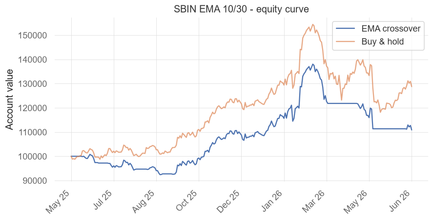
Save the equity curve
Numbers persuade the head; a picture persuades the gut. We plot the strategy's equity curve against buy-and-hold and save it as a PNG with matplotlib. (The portal embeds any PNG saved next to an example automatically.)
# Save the strategy's equity curve next to buy-and-hold as a PNG.
import datetime
import os
from pathlib import Path

import matplotlib

matplotlib.use("Agg")
import matplotlib.pyplot as plt
import vectorbt as vbt
from openalgo import api, ta

client = api(
    api_key=os.getenv("OPENALGO_API_KEY", "your_api_key_here"),
    host=os.getenv("OPENALGO_HOST", "http://127.0.0.1:5000"),
)

end = datetime.date.today()
start = end - datetime.timedelta(days=400)
df = client.history(symbol="SBIN", exchange="NSE", interval="D",
                    start_date=str(start), end_date=str(end))
close = df["close"].astype(float)
fast, slow = ta.ema(close, 10), ta.ema(close, 30)
entries = (fast > slow) & (fast.shift(1) <= slow.shift(1))
exits = (fast < slow) & (fast.shift(1) >= slow.shift(1))
pf = vbt.Portfolio.from_signals(close, entries, exits,
                                init_cash=100000, fees=0.001, slippage=0.0005, freq="1D")

equity = pf.value()                                   # strategy account value
buyhold = 100000 * (close / close.iloc[0])            # buy-and-hold value
x = list(range(len(equity)))                          # positional x, no gaps
fig, ax = plt.subplots(figsize=(9, 4))
ax.plot(x, equity.values, label="EMA crossover")
ax.plot(x, buyhold.values, label="Buy & hold", alpha=0.7)
ax.set_title("SBIN EMA 10/30 - equity curve"); ax.set_ylabel("Account value"); ax.legend()
step = max(1, len(equity) // 8)
ax.set_xticks(x[::step])
ax.set_xticklabels(equity.index[::step].strftime("%b %y"), rotation=45, ha="right")
out = Path(__file__).with_suffix(".png")
fig.savefig(out, dpi=110, bbox_inches="tight")
print(f"Saved {out.name}")Saved 09_equity_curve_png.png
It works on anything
A backtest doesn't care what it's testing - feed it any price series and the workflow is identical. Here's the exact same EMA-crossover machinery applied to a gold future on MCX, with a slightly slower 20/50 pair to suit a smoother-trending commodity.
# The same workflow on an MCX commodity future - backtesting is asset-agnostic.
import datetime
import os

import vectorbt as vbt
from openalgo import api, ta

client = api(
    api_key=os.getenv("OPENALGO_API_KEY", "your_api_key_here"),
    host=os.getenv("OPENALGO_HOST", "http://127.0.0.1:5000"),
)

end = datetime.date.today()
start = end - datetime.timedelta(days=400)
df = client.history(symbol="GOLDM03JUL26FUT", exchange="MCX", interval="D",
                    start_date=str(start), end_date=str(end))
close = df["close"].astype(float)

# Gold trends well, so use a slightly slower pair (20/50).
fast, slow = ta.ema(close, 20), ta.ema(close, 50)
entries = (fast > slow) & (fast.shift(1) <= slow.shift(1))
exits = (fast < slow) & (fast.shift(1) >= slow.shift(1))
pf = vbt.Portfolio.from_signals(close, entries, exits,
                                init_cash=200000, fees=0.0005, slippage=0.0005, freq="1D")

print(f"Bars              : {len(close)}")
print(f"GOLDM total return: {pf.total_return() * 100:.2f}%")
print(f"Buy & hold return : {(close.iloc[-1] / close.iloc[0] - 1) * 100:.2f}%")
print(f"Max drawdown      : {pf.max_drawdown() * 100:.2f}%")
print(f"Trades : {pf.trades.count()}")Bars : 120 GOLDM total return: -11.43% Buy & hold return : -3.05% Max drawdown : -32.04% Trades : 2
Try it yourself
- Change the EMA pair from 10/30 to 20/50 on the NSE stock. Does it trade less? Does it beat buy-and-hold?
- Re-run the VectorBT portfolio with
fees=0and compare the total return - how much did costs eat? - Swap the stock in any example for one you follow and read its
pf.stats()benchmark line: did the strategy add value over simply holding?
Recap
- A backtest replays a strategy on history so you can judge an edge before risking money.
- By hand: signal -> position with
.shift(1)(the cure for look-ahead bias) -> strategy return =position * market_return-> equity curve via(1 + returns).cumprod(). - VectorBT reproduces all of this fast, in events:
entriesandexitsfed tovbt.Portfolio.from_signals(...). - Always include realistic costs (
fees,slippage) - they can turn a paper winner into a real loser. pf.stats()is the one-glance report card;direction="both"lets the strategy go short as well as long.- The workflow is asset-agnostic - the same code backtests an NSE stock or an MCX commodity.
Your strategy now has an equity curve and a pile of numbers. But which numbers actually tell you whether it's good? Next we decode them - CAGR, Sharpe, Sortino, drawdown, win rate and more - and benchmark the strategy properly against the index.