Module G · Backtesting & Optimisation - Chapter 28

Parameter Optimisation

Sweep parameter grids, draw heatmaps and pick robust settings - not just the best.

NSEMCX

What you'll learn

·Define a param grid
·VectorBT broadcasting
·Returns heatmap
·Sharpe heatmap
·Robust vs peak
·Cost-aware optimisation

In the last two chapters you learned to backtest a single strategy and to score it with Sharpe, drawdown and the rest. But every strategy has knobs. An EMA crossover asks: how fast is the fast line? how slow is the slow one? A Bollinger system asks how many standard deviations. Change a knob and the equity curve changes with it. So the obvious question lands almost immediately: which settings are best?

This chapter answers that question - and then, more importantly, teaches you to distrust the answer. Finding the single highest-scoring parameter combination is easy and almost always a trap. The real skill is finding a region of settings that all work, because that is what survives contact with next year's market. We'll sweep a grid of parameters with VectorBT, draw heatmaps to see the whole landscape at once, and learn to tell a genuine edge from a lucky fluke.

What optimisation really is

Parameter optimisation is just trying many settings and comparing the results. That's it. There's no magic - you pick a few values for each knob, test every combination on your history, and rank them by some score (return, Sharpe, whatever you care about).

The set of combinations you test is called a grid. If you try four fast EMA lengths and four slow ones, that's sixteen pairs - a 4x4 grid. Keep grids small to start. Every extra value you add multiplies the work and multiplies the number of chances for one combo to look brilliant purely by luck.

EX 1Build a small parameter gridch28/01_param_grid.py

# An optimisation starts with a parameter GRID -- every combo we want to test.
import itertools

# A grid is just the set of settings you want to try.
fast_lengths = [10, 20, 30, 40]      # fast EMA candidates
slow_lengths = [20, 30, 40, 50]      # slow EMA candidates

# A "combo" is one (fast, slow) pair. We only keep pairs where fast < slow,
# because a crossover system needs the fast line to be the quicker one. The
# ranges overlap, so several raw pairs (e.g. 40/20) are nonsense and get cut.
combos = [(f, s) for f, s in itertools.product(fast_lengths, slow_lengths) if f < s]

print(f"Fast options : {fast_lengths}")
print(f"Slow options : {slow_lengths}")
print(f"Raw combos   : {len(fast_lengths) * len(slow_lengths)}")
print(f"Valid combos : {len(combos)}  (kept only fast < slow)")
print("\nFirst few combos to test:")
for f, s in combos[:5]:
    print(f"  EMA {f} crossing EMA {s}")

# Keep grids small. Each extra value multiplies the work -- and the temptation
# to cherry-pick a winner that only looks good by luck.

Live output

Fast options : [10, 20, 30, 40]
Slow options : [20, 30, 40, 50]
Raw combos   : 16
Valid combos : 10  (kept only fast < slow)

First few combos to test:
  EMA 10 crossing EMA 20
  EMA 10 crossing EMA 30
  EMA 10 crossing EMA 40
  EMA 10 crossing EMA 50
  EMA 20 crossing EMA 30

Tip

Notice we keep only combos where the fast length is genuinely smaller than the slow one. Because the candidate ranges overlap, several pairs in the raw 4x4 grid are nonsense for a crossover system (you can't have the "fast" line be slower than the "slow" line), so we filter them out before wasting any compute on them.

One combo, one set of signals

Before sweeping everything, let's be crystal clear about the unit we're repeating. For one (fast, slow) pair we compute two EMAs, then mark an entry the day the fast line crosses above the slow one, and an exit the day it crosses back below. That shift(1) is doing real work: it compares today's relationship to yesterday's, so we fire only on the day of the cross, not on every day the fast line happens to be on top.

EX 2Signals for a single comboNSEch28/02_signals_per_combo.py

# Turn one (fast, slow) combo into entry/exit signals -- the unit we repeat.
import os
from datetime import datetime, timedelta

from openalgo import api, ta

client = api(
    api_key=os.getenv("OPENALGO_API_KEY", "your_api_key_here"),
    host=os.getenv("OPENALGO_HOST", "http://127.0.0.1:5000"),
)

end = datetime.now().strftime("%Y-%m-%d")
start = (datetime.now() - timedelta(days=500)).strftime("%Y-%m-%d")
df = client.history(symbol="RELIANCE", exchange="NSE", interval="D", start_date=start, end_date=end)
close = df["close"]

fast, slow = 10, 50
fast_ema = ta.ema(close, fast)
slow_ema = ta.ema(close, slow)

# Enter when the fast EMA crosses ABOVE the slow; exit when it crosses below.
entries = (fast_ema > slow_ema) & (fast_ema.shift(1) <= slow_ema.shift(1))
exits = (fast_ema < slow_ema) & (fast_ema.shift(1) >= slow_ema.shift(1))

print(f"EMA {fast} / {slow} on RELIANCE, {len(close)} daily bars")
print(f"Entry signals: {int(entries.sum())}")
print(f"Exit signals : {int(exits.sum())}")
print("\nWe will run this exact recipe for every combo in the grid.")

Live output

EMA 10 / 50 on RELIANCE, 336 daily bars
Entry signals: 4
Exit signals : 5

We will run this exact recipe for every combo in the grid.

This is exactly the kind of signal you built in Chapter 17. Optimisation doesn't change how you make signals - it just runs the same recipe many times with different numbers.

Sweeping the whole grid in one call

Here's where VectorBT earns its keep. Instead of looping and running sixteen separate backtests, we build a 2D signal table: rows are dates, and each column is one combo. Pass those two tables (entries and exits) to Portfolio.from_signals once, and VectorBT backtests all sixteen strategies in a single vectorised sweep. The result, pf.total_return(), comes back as one number per column - a Series indexed by your (fast, slow) pairs.

EX 3Sweep every combo with VectorBTNSEch28/03_sweep_vectorbt.py

# Broadcast every combo into 2D signals and backtest them all in ONE VectorBT call.
import os
from datetime import datetime, timedelta

import pandas as pd
import vectorbt as vbt
from openalgo import api, ta

client = api(
    api_key=os.getenv("OPENALGO_API_KEY", "your_api_key_here"),
    host=os.getenv("OPENALGO_HOST", "http://127.0.0.1:5000"),
)

end = datetime.now().strftime("%Y-%m-%d")
start = (datetime.now() - timedelta(days=500)).strftime("%Y-%m-%d")
df = client.history(symbol="RELIANCE", exchange="NSE", interval="D", start_date=start, end_date=end)
close = df["close"]

combos = [(f, s) for f in (5, 10, 15, 20) for s in (30, 40, 50, 60) if f < s]
ent, ext = {}, {}
for f, s in combos:                                   # one column per combo
    fe, se = ta.ema(close, f), ta.ema(close, s)
    ent[(f, s)] = (fe > se) & (fe.shift(1) <= se.shift(1))
    ext[(f, s)] = (fe < se) & (fe.shift(1) >= se.shift(1))

cols = pd.MultiIndex.from_tuples(combos, names=["fast", "slow"])
entries = pd.DataFrame(ent).set_axis(cols, axis=1)    # 2D: rows=dates, cols=combos
exits = pd.DataFrame(ext).set_axis(cols, axis=1)

pf = vbt.Portfolio.from_signals(close, entries, exits, init_cash=100000, fees=0.001, freq="1D")
ret = pf.total_return().sort_values(ascending=False)  # one return per combo
print(f"Tested {len(combos)} combos in a single backtest.\n")
print("Best 3 combos by total return:")
print((ret.head(3) * 100).round(2).astype(str) + " %")

Live output

Tested 16 combos in a single backtest.

Best 3 combos by total return:
fast  slow
5     40       3.1 %
      30      2.98 %
      50      2.28 %
Name: total_return, dtype: object

Key idea

The trick is the column MultiIndex: pd.MultiIndex.from_tuples(combos, names=["fast", "slow"]). It labels each column with its two parameters at once. That's what lets us later unstack("slow") to reshape the flat results into a 2D grid for a heatmap. Learn this pattern - it's the backbone of every optimisation you'll run.

A word on what these numbers mean. We're testing on RELIANCE over roughly 500 calendar days of daily bars, with a realistic 0.1% fee per trade. Crossover systems on a single stock won't shoot the lights out - and that's fine. The point of this chapter is the method, not the headline return.

Seeing the landscape: heatmaps

A ranked list tells you the winner but hides the shape. A heatmap shows the whole terrain - a coloured grid where green is good and red is bad. Suddenly you can see whether the good results huddle together in a region or sit alone like a single lucky pixel.

We reshape the flat results with .unstack("slow") so fast lengths run down the rows and slow lengths across the columns, then draw it with matplotlib's imshow and save it as a PNG.

A returns heatmap chart — EX 4A returns heatmapNSEch28/04_returns_heatmap.py

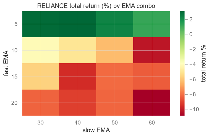
Total return is seductive but incomplete: a combo can post a big number while putting you through gut-wrenching swings to get there. Sharpe divides return by volatility, so it rewards smooth growth. Drawing the same grid coloured by Sharpe often points you somewhere different - and usually somewhere you'd actually be willing to trade.

A Sharpe heatmap chart — EX 5A Sharpe heatmapNSEch28/05_sharpe_heatmap.py

Note

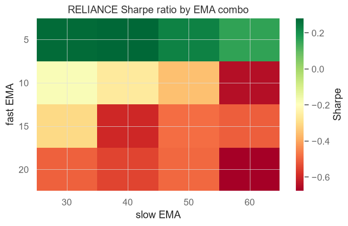
Both examples save a .png next to the script, and the portal embeds it automatically. Open them side by side: the combo with the highest return is frequently not the one with the highest Sharpe. Which would you rather trade - the one that made slightly more, or the one that let you sleep at night?

The single biggest mistake: chasing the peak

Now the lesson that separates people who make money from people who only make backtests. The highest-scoring combo on your history is almost certainly overfit - tuned so tightly to the past that it has memorised noise rather than learned a pattern. Overfitting means your strategy has fit the random wiggles of this specific history, wiggles that will never repeat. Trade it live and the edge evaporates.

The defence is to look at the neighbourhood. A trustworthy setting is one whose neighbours on the heatmap also score well - a broad green plateau, not a lonely green dot in a sea of red. If EMA 12/48 is great but 11/48 and 13/48 are terrible, you haven't found an edge; you've found a coincidence. A robust plateau means that even if the perfect lengths drift a little next year, you're still standing on solid ground.

EX 6Robust region vs the lonely peakNSEch28/06_robust_vs_peak.py

# The single best combo is often LUCK. A robust region beats a lonely peak.
import os
from datetime import datetime, timedelta

import pandas as pd
import vectorbt as vbt
from openalgo import api, ta

client = api(
    api_key=os.getenv("OPENALGO_API_KEY", "your_api_key_here"),
    host=os.getenv("OPENALGO_HOST", "http://127.0.0.1:5000"),
)

end = datetime.now().strftime("%Y-%m-%d")
start = (datetime.now() - timedelta(days=500)).strftime("%Y-%m-%d")
close = client.history(symbol="RELIANCE", exchange="NSE", interval="D",
                       start_date=start, end_date=end)["close"]

combos = [(f, s) for f in (5, 10, 15, 20) for s in (30, 40, 50, 60) if f < s]
ent, ext = {}, {}
for f, s in combos:
    fe, se = ta.ema(close, f), ta.ema(close, s)
    ent[(f, s)] = (fe > se) & (fe.shift(1) <= se.shift(1))
    ext[(f, s)] = (fe < se) & (fe.shift(1) >= se.shift(1))
cols = pd.MultiIndex.from_tuples(combos, names=["fast", "slow"])
pf = vbt.Portfolio.from_signals(close, pd.DataFrame(ent).set_axis(cols, axis=1),
                                pd.DataFrame(ext).set_axis(cols, axis=1),
                                init_cash=100000, fees=0.001, freq="1D")

grid = pf.sharpe_ratio().unstack("slow")
peak = pf.sharpe_ratio().idxmax()
# A combo is only trustworthy if its NEIGHBOURS also score well. We grade each
# combo by the average Sharpe of its local block (itself plus adjacent cells).
smoothed = grid.rolling(2, min_periods=1).mean().T.rolling(2, min_periods=1).mean().T
robust = smoothed.stack().idxmax()

print(f"Lonely peak (best single combo) : EMA {peak[0]}/{peak[1]}")
print(f"Robust pick (best neighbourhood): EMA {robust[0]}/{robust[1]}")
print("\nPrefer a setting surrounded by other good settings: if next year the")
print("ideal lengths drift a little, you are still standing on solid ground.")

Live output

Lonely peak (best single combo) : EMA 5/40
Robust pick (best neighbourhood): EMA 5/40

Prefer a setting surrounded by other good settings: if next year the
ideal lengths drift a little, you are still standing on solid ground.

Heads up

Red flags that you're overfitting: the best combo beats its neighbours by a mile; tiny parameter changes flip the result from great to awful; the "winner" took very few trades (a handful of lucky entries can fake a wonderful curve). When you see these, trust the robust region, not the peak - and read Chapter 29 on walk-forward testing before you risk a rupee.

Optimise with costs, or fool yourself

One more way to lie to yourself: optimising as if trading were free. Fast combos trade more often, and every trade pays brokerage, taxes and slippage. A frictionless backtest will happily crown a hyperactive setting that real costs would bleed dry. So you must include realistic costs inside the optimisation - the moment you account for them, the ranking can shift toward calmer, lower-turnover settings.

EX 7Cost-aware optimisationNSEch28/07_cost_aware.py

# Costs change the winner. Optimise WITH realistic fees, never on a frictionless dream.
import os
from datetime import datetime, timedelta

import pandas as pd
import vectorbt as vbt
from openalgo import api, ta

client = api(
    api_key=os.getenv("OPENALGO_API_KEY", "your_api_key_here"),
    host=os.getenv("OPENALGO_HOST", "http://127.0.0.1:5000"),
)

end = datetime.now().strftime("%Y-%m-%d")
start = (datetime.now() - timedelta(days=500)).strftime("%Y-%m-%d")
close = client.history(symbol="RELIANCE", exchange="NSE", interval="D",
                       start_date=start, end_date=end)["close"]

combos = [(f, s) for f in (5, 10, 15, 20) for s in (30, 40, 50, 60) if f < s]
ent, ext = {}, {}
for f, s in combos:
    fe, se = ta.ema(close, f), ta.ema(close, s)
    ent[(f, s)] = (fe > se) & (fe.shift(1) <= se.shift(1))
    ext[(f, s)] = (fe < se) & (fe.shift(1) >= se.shift(1))
cols = pd.MultiIndex.from_tuples(combos, names=["fast", "slow"])
entries = pd.DataFrame(ent).set_axis(cols, axis=1)
exits = pd.DataFrame(ext).set_axis(cols, axis=1)

# Same signals, two cost assumptions. fees=0.0015 ~ 0.15% per trade (brokerage + taxes).
free = vbt.Portfolio.from_signals(close, entries, exits, init_cash=100000, fees=0.0, freq="1D")
real = vbt.Portfolio.from_signals(close, entries, exits, init_cash=100000,
                                  fees=0.0015, slippage=0.0005, freq="1D")

best_free = tuple(int(x) for x in free.total_return().idxmax())
best_real = tuple(int(x) for x in real.total_return().idxmax())
print(f"Best combo with NO costs  : EMA {best_free[0]}/{best_free[1]}")
print(f"Best combo WITH costs     : EMA {best_real[0]}/{best_real[1]}")
fast_combo = (5, 30)
print(f"\nFor the trade-heavy EMA {fast_combo[0]}/{fast_combo[1]}:")
print(f"  return no-cost : {free.total_return()[fast_combo] * 100:6.2f} %")
print(f"  return costed  : {real.total_return()[fast_combo] * 100:6.2f} %  <- fees punish churn")

Live output

Best combo with NO costs  : EMA 5/30
Best combo WITH costs     : EMA 5/40

For the trade-heavy EMA 5/30:
  return no-cost :   4.23 %
  return costed  :   1.76 %  <- fees punish churn

See how the trade-heavy EMA 5/30 looks fine with zero costs but limps once fees and slippage bite? That's the churn tax. Optimising with fees=... and slippage=... set to realistic numbers is non-negotiable.

A different market: gold on MCX

Finally, a reminder that an edge is asset-specific. The settings that suit a large-cap stock need not suit a commodity that trends and ranges on its own rhythm. Here we run the identical sweep on MCX gold-mini futures and compare the table - the best combo is frequently not the one that won on the stock.

EX 8Optimise gold futures on MCXMCXch28/08_mcx_optimize.py

# Same sweep, a different market: gold futures on MCX. Edges are asset-specific.
import os
from datetime import datetime, timedelta

import pandas as pd
import vectorbt as vbt
from openalgo import api, ta

client = api(
    api_key=os.getenv("OPENALGO_API_KEY", "your_api_key_here"),
    host=os.getenv("OPENALGO_HOST", "http://127.0.0.1:5000"),
)

end = datetime.now().strftime("%Y-%m-%d")
start = (datetime.now() - timedelta(days=400)).strftime("%Y-%m-%d")
# GOLDM = mini gold contract on MCX. Commodities trend differently from equities.
close = client.history(symbol="GOLDM03JUL26FUT", exchange="MCX", interval="D",
                       start_date=start, end_date=end)["close"]

combos = [(f, s) for f in (5, 10, 20) for s in (30, 50) if f < s]
ent, ext = {}, {}
for f, s in combos:
    fe, se = ta.ema(close, f), ta.ema(close, s)
    ent[(f, s)] = (fe > se) & (fe.shift(1) <= se.shift(1))
    ext[(f, s)] = (fe < se) & (fe.shift(1) >= se.shift(1))
cols = pd.MultiIndex.from_tuples(combos, names=["fast", "slow"])
pf = vbt.Portfolio.from_signals(close, pd.DataFrame(ent).set_axis(cols, axis=1),
                                pd.DataFrame(ext).set_axis(cols, axis=1),
                                init_cash=200000, fees=0.0008, freq="1D")

table = pd.DataFrame({"return_%": (pf.total_return() * 100).round(2),
                      "sharpe": pf.sharpe_ratio().round(2)}).sort_values("sharpe", ascending=False)
print(f"GOLDM gold futures, {len(close)} daily bars on MCX\n")
print(table)
print("\nNote how the best settings here need not match RELIANCE -- never assume")
print("one parameter set is universal. Re-optimise per instrument.")

Live output

GOLDM gold futures, 120 daily bars on MCX

           return_%  sharpe
fast slow                  
5    30        3.68    0.48
     50       -7.72   -0.41
10   50       -8.21   -0.45
     30       -8.82   -0.50
20   30       -9.46   -0.55
     50      -11.36   -0.70

Note how the best settings here need not match RELIANCE -- never assume
one parameter set is universal. Re-optimise per instrument.

The takeaway: never assume one parameter set is universal. Re-run your optimisation per instrument, and per market regime, and treat every "best" with healthy suspicion.

Try it yourself

Widen the grid in 03_sweep_vectorbt.py to fast [5, 8, 11, 14] and slow [25, 35, 45, 55]. Does a clearer plateau appear in the heatmap, or just more noise?
In the cost-aware example, push fees to 0.003 (0.3%). Which combos survive the higher tax, and what does that tell you about turnover?
Swap RELIANCE for a stock you follow, regenerate the Sharpe heatmap, and decide which region you'd actually trade - and why.

Recap

Optimisation is simply testing a grid of parameter combinations and ranking them - keep grids small.
VectorBT sweeps every combo in one call when you pass 2D entries/exits with a (fast, slow) column MultiIndex.
Heatmaps reveal the whole landscape; a Sharpe heatmap often disagrees with a return heatmap, and Sharpe is usually the wiser guide.
Chasing the single highest peak is overfitting - prefer a robust region whose neighbours also score well.
Always optimise with realistic costs; free backtests reward churn that real fees would punish.
An edge is asset-specific - re-optimise per instrument rather than trusting one universal setting.

Heatmaps show us the best settings on the past. But the past is exactly what we risk overfitting to. Next chapter we build the proper antidote: walk-forward testing, where we tune on one slice of history and judge the result on a slice the strategy has never seen.