Machine Learning, Neural Nets & a Complete Bot
Engineer features, train a classifier and a neural network, then wire it into a live OpenAlgo loop.
- ·Features from indicators
- ·Train/test for ML
- ·Logistic & random forest
- ·A neural network (MLP)
- ·Walk-forward ML check
- ·End-to-end trading bot
You've arrived at the final chapter, and you've earned a different kind of tool. Everything so far has been you writing the rules: cross this average, exit on that signal, optimise these lengths. Machine learning flips that around. Instead of telling the computer the rule, you show it thousands of examples and let it find the rule itself. Then we take that learned model, wrap it in code that fetches data and places orders, and end the series the way we promised in Chapter 1 - with a complete, runnable bot.
Let's demystify ML before we touch it, because the hype around it is enormous and mostly unhelpful for traders. A machine learning model is just a function that takes some numbers in (your indicators) and gives a guess out (will the next bar go up?). It "learns" by looking at historical examples where the answer is already known, and adjusting itself until its guesses match those answers as often as possible. That's the whole magic. No intuition, no understanding of markets - just pattern-matching on numbers. Which means the quality of your numbers, and the honesty of your testing, matter far more than which fancy model you pick.
A blunt warning up front: predicting next-bar direction is genuinely hard, and the honest accuracy you'll see in this chapter hovers near a coin flip. That is not a bug in your code - it's the reality of efficient markets. The goal here is to learn the ML workflow correctly, not to discover a money machine. Anyone selling you a model that "predicts the market with 90% accuracy" is selling you an overfitted fantasy.
Features: the clues you hand the model
A feature is one numeric clue the model gets to look at. A model can't read a chart; it reads columns of numbers. So our first job - and the one that matters most - is feature engineering: turning raw OHLCV into a tidy table of informative numbers. Everything you learned about indicators pays off here. RSI captures momentum, ATR captures volatility, the distance from an EMA captures how stretched price is from its trend, and recent returns capture short-term drift.
# Feature engineering: turn raw prices into the columns a model can learn from.
import os
from datetime import datetime, timedelta

import pandas as pd
from openalgo import api, ta

client = api(
    api_key=os.getenv("OPENALGO_API_KEY", "your_api_key_here"),
    host=os.getenv("OPENALGO_HOST", "http://127.0.0.1:5000"),
)

end = datetime.now().strftime("%Y-%m-%d")
start = (datetime.now() - timedelta(days=900)).strftime("%Y-%m-%d")
df = client.history(symbol="RELIANCE", exchange="NSE", interval="D", start_date=start, end_date=end)
c = df["close"]

# A "feature" is one numeric clue the model reads. We build a table of them.
feat = pd.DataFrame(index=df.index)
feat["rsi"] = ta.rsi(c, 14)                       # momentum: overbought / oversold
feat["ret1"] = c.pct_change()                     # yesterday's return
feat["ret5"] = c.pct_change(5)                    # one-week return
feat["atr"] = ta.atr(df["high"], df["low"], c, 14)  # volatility (range size)
feat["ema_dist"] = (c - ta.ema(c, 20)) / c        # how far price is from its trend
feat = feat.dropna()                              # drop warm-up rows with no value yet

print(f"Built {feat.shape[1]} features over {feat.shape[0]} usable bars.")
print("\nLast 3 rows of the feature table:")
print(feat.tail(3).round(4))Built 5 features over 596 usable bars.
Last 3 rows of the feature table:
rsi ret1 ret5 atr ema_dist
timestamp
2026-06-19 46.1465 -0.0140 0.0128 26.7868 -0.0051
2026-06-22 50.9139 0.0130 0.0149 27.4020 0.0071
2026-06-23 45.6642 -0.0155 -0.0172 27.5162 -0.0077Notice we dropna() at the end. Indicators need a warm-up period (a 14-day RSI has no value on day 3), so the early rows are blank and must go. A model can't learn from missing numbers.
The label: what we're trying to predict
If features are the question, the label (or target) is the answer we want the model to learn. Here we ask the simplest useful question in trading: will the next bar close higher than this one? We build the label with c.shift(-1) > c - shift(-1) pulls tomorrow's close back onto today's row, so each row pairs today's features with tomorrow's outcome.
# The LABEL: what we want the model to predict -- did the NEXT bar close up?
import os
from datetime import datetime, timedelta

import pandas as pd
from openalgo import api, ta

client = api(
    api_key=os.getenv("OPENALGO_API_KEY", "your_api_key_here"),
    host=os.getenv("OPENALGO_HOST", "http://127.0.0.1:5000"),
)

end = datetime.now().strftime("%Y-%m-%d")
start = (datetime.now() - timedelta(days=900)).strftime("%Y-%m-%d")
df = client.history(symbol="RELIANCE", exchange="NSE", interval="D", start_date=start, end_date=end)
c = df["close"]

data = pd.DataFrame(index=df.index)
data["rsi"] = ta.rsi(c, 14)
data["ret1"] = c.pct_change()
# Label = 1 if TOMORROW closes higher than today, else 0. shift(-1) looks one bar ahead.
data["target"] = (c.shift(-1) > c).astype(int)
data = data.dropna()

up = int(data["target"].sum())
print(f"Rows: {len(data)}   up days: {up}   down days: {len(data) - up}")
print(f"Base rate (share of up days): {up / len(data):.1%}")
print("\nThat base rate is the score to beat -- always guessing 'up' would hit it.")
print("A model is only useful if it beats this naive baseline out-of-sample.")Rows: 596 up days: 296 down days: 300 Base rate (share of up days): 49.7% That base rate is the score to beat -- always guessing 'up' would hit it. A model is only useful if it beats this naive baseline out-of-sample.
That base rate - the share of up days - is the number to beat. If 53% of days are up, a lazy model that always shouts "up" scores 53%. So when your sophisticated neural network scores 52%, it is actually worse than guessing. Always compare model accuracy to this naive baseline; accuracy in isolation is meaningless.
Train and test: the cardinal rule
You met this idea in Chapter 29 and it's even more vital here. We split our table into a training set (where the model learns) and a test set (where we grade it on data it never saw). For time-series data we always pass shuffle=False, so training is strictly the past and testing is strictly the future. Shuffling would let the model peek at tomorrow while learning from today - a subtle leak that makes a useless model look brilliant.
# Split features+label into train/test -- shuffle=False, because time has an order.
import os
from datetime import datetime, timedelta

import pandas as pd
from openalgo import api, ta
from sklearn.model_selection import train_test_split

client = api(
    api_key=os.getenv("OPENALGO_API_KEY", "your_api_key_here"),
    host=os.getenv("OPENALGO_HOST", "http://127.0.0.1:5000"),
)

end = datetime.now().strftime("%Y-%m-%d")
start = (datetime.now() - timedelta(days=900)).strftime("%Y-%m-%d")
df = client.history(symbol="RELIANCE", exchange="NSE", interval="D", start_date=start, end_date=end)
c = df["close"]

d = pd.DataFrame(index=df.index)
d["rsi"] = ta.rsi(c, 14)
d["ret1"] = c.pct_change()
d["target"] = (c.shift(-1) > c).astype(int)
d = d.dropna()

X = d[["rsi", "ret1"]]                             # the clues (features)
y = d["target"]                                    # the answer (label)
# shuffle=False keeps the split chronological: train on the past, test on the future.
X_train, X_test, y_train, y_test = train_test_split(X, y, test_size=0.25, shuffle=False)

print(f"Train rows: {len(X_train)}  ({X_train.index[0].date()} -> {X_train.index[-1].date()})")
print(f"Test rows : {len(X_test)}  ({X_test.index[0].date()} -> {X_test.index[-1].date()})")
print("\nThe model learns on train and is graded on test -- data it never saw.")Train rows: 447 (2024-01-25 -> 2025-11-13) Test rows : 149 (2025-11-14 -> 2026-06-23) The model learns on train and is graded on test -- data it never saw.
Two classic models: logistic regression and random forest
Time to actually learn something. We'll start with two workhorses from scikit-learn:
- Logistic Regression - despite the name, it's a classifier. It draws the best straight-line boundary between "up" and "down" in feature space. Simple, fast, and a sane first baseline.
- Random Forest - a crowd of decision trees, each asking yes/no questions about the features ("is RSI above 60? is ATR rising?"), then voting. It captures curved, interacting patterns a straight line can't.
Both follow the same three-word ritual you'll use for every scikit-learn model: .fit() to learn, .predict() to guess, then score with accuracy_score.
# Two classic models: Logistic Regression and a Random Forest. Report accuracy.
import os
from datetime import datetime, timedelta

import pandas as pd
from openalgo import api, ta
from sklearn.ensemble import RandomForestClassifier
from sklearn.linear_model import LogisticRegression
from sklearn.metrics import accuracy_score
from sklearn.model_selection import train_test_split

client = api(
    api_key=os.getenv("OPENALGO_API_KEY", "your_api_key_here"),
    host=os.getenv("OPENALGO_HOST", "http://127.0.0.1:5000"),
)

end = datetime.now().strftime("%Y-%m-%d")
start = (datetime.now() - timedelta(days=900)).strftime("%Y-%m-%d")
df = client.history(symbol="RELIANCE", exchange="NSE", interval="D", start_date=start, end_date=end)
c = df["close"]
d = pd.DataFrame(index=df.index)
d["rsi"] = ta.rsi(c, 14); d["ret1"] = c.pct_change(); d["ret5"] = c.pct_change(5)
d["atr"] = ta.atr(df["high"], df["low"], c, 14); d["ema_dist"] = (c - ta.ema(c, 20)) / c
d["target"] = (c.shift(-1) > c).astype(int)
d = d.dropna()

X, y = d.drop(columns="target"), d["target"]
Xtr, Xte, ytr, yte = train_test_split(X, y, test_size=0.25, shuffle=False)
base = max(yte.mean(), 1 - yte.mean())              # naive "always pick the common class"

logit = LogisticRegression(max_iter=1000).fit(Xtr, ytr)
forest = RandomForestClassifier(n_estimators=100, max_depth=4, random_state=0).fit(Xtr, ytr)
print(f"Naive baseline      : {base:.1%}")
print(f"Logistic Regression : {accuracy_score(yte, logit.predict(Xte)):.1%}")
print(f"Random Forest       : {accuracy_score(yte, forest.predict(Xte)):.1%}")
print("\nNext-bar direction is HARD: scores near the baseline are the honest norm.")Naive baseline : 54.4% Logistic Regression : 47.0% Random Forest : 47.7% Next-bar direction is HARD: scores near the baseline are the honest norm.
Don't be disappointed by scores hugging the baseline. That's the honest result, and seeing it teaches you more than a faked 90% ever would.
The neural network
Now the star everyone asks about. A neural network is a model loosely inspired by brain cells: layers of simple units ("neurons"), each combining its inputs and passing the result to the next layer. Stack enough layers and the network can, in principle, learn very complex, twisty patterns. In scikit-learn it's the MLPClassifier (MLP = multi-layer perceptron), and hidden_layer_sizes=(16, 8) means two hidden layers of 16 and 8 neurons.
One new step matters: neural nets are sensitive to the scale of their inputs, so we standardise the features with StandardScaler - and we fit the scaler on the training data only, then apply it to the test data. Fitting it on everything would leak information from the future.
# The NEURAL NETWORK: an MLPClassifier. Same job, layered "neurons" inside.
import os
from datetime import datetime, timedelta

import pandas as pd
from openalgo import api, ta
from sklearn.metrics import accuracy_score
from sklearn.model_selection import train_test_split
from sklearn.neural_network import MLPClassifier
from sklearn.preprocessing import StandardScaler

client = api(
    api_key=os.getenv("OPENALGO_API_KEY", "your_api_key_here"),
    host=os.getenv("OPENALGO_HOST", "http://127.0.0.1:5000"),
)

end = datetime.now().strftime("%Y-%m-%d")
start = (datetime.now() - timedelta(days=900)).strftime("%Y-%m-%d")
df = client.history(symbol="RELIANCE", exchange="NSE", interval="D", start_date=start, end_date=end)
c = df["close"]
d = pd.DataFrame(index=df.index)
d["rsi"] = ta.rsi(c, 14); d["ret1"] = c.pct_change(); d["ret5"] = c.pct_change(5)
d["atr"] = ta.atr(df["high"], df["low"], c, 14); d["ema_dist"] = (c - ta.ema(c, 20)) / c
d["target"] = (c.shift(-1) > c).astype(int)
d = d.dropna()

X, y = d.drop(columns="target"), d["target"]
Xtr, Xte, ytr, yte = train_test_split(X, y, test_size=0.25, shuffle=False)
# Neural nets need features on a similar scale -- fit the scaler on TRAIN only.
scaler = StandardScaler().fit(Xtr)
Xtr_s, Xte_s = scaler.transform(Xtr), scaler.transform(Xte)

# hidden_layer_sizes=(16, 8): two hidden layers of 16 and 8 neurons.
mlp = MLPClassifier(hidden_layer_sizes=(16, 8), max_iter=1000, random_state=0).fit(Xtr_s, ytr)
print(f"Naive baseline : {max(yte.mean(), 1 - yte.mean()):.1%}")
print(f"Neural net (MLP): {accuracy_score(yte, mlp.predict(Xte_s)):.1%}")
print("\nMore layers can fit more complex patterns -- and overfit faster. Bigger is not safer.")Naive baseline : 54.4% Neural net (MLP): 49.0% More layers can fit more complex patterns -- and overfit faster. Bigger is not safer.
More neurons and more layers do not mean a better trader. A bigger network fits the training data more tightly - including its random noise - and overfits faster. On the small, noisy datasets of single-stock trading, simple models often beat complex ones out-of-sample. Reach for capacity only when more data and honest testing justify it.
Which clues mattered? Feature importance
A trained Random Forest can tell you which features it actually leaned on - its feature importance. This is one of the most practical things ML offers a trader: it's a data-driven hint about what's predictive and what's just dead weight you can drop. We plot the importances and save the chart as a PNG.
# Which clues mattered? A Random Forest ranks its features by importance.
import os
from datetime import datetime, timedelta
from pathlib import Path

import matplotlib.pyplot as plt
import pandas as pd
from openalgo import api, ta
from sklearn.ensemble import RandomForestClassifier
from sklearn.model_selection import train_test_split

client = api(
    api_key=os.getenv("OPENALGO_API_KEY", "your_api_key_here"),
    host=os.getenv("OPENALGO_HOST", "http://127.0.0.1:5000"),
)

end = datetime.now().strftime("%Y-%m-%d")
start = (datetime.now() - timedelta(days=900)).strftime("%Y-%m-%d")
df = client.history(symbol="RELIANCE", exchange="NSE", interval="D", start_date=start, end_date=end)
c = df["close"]
d = pd.DataFrame(index=df.index)
d["rsi"] = ta.rsi(c, 14); d["ret1"] = c.pct_change(); d["ret5"] = c.pct_change(5)
d["atr"] = ta.atr(df["high"], df["low"], c, 14); d["ema_dist"] = (c - ta.ema(c, 20)) / c
d["target"] = (c.shift(-1) > c).astype(int)
d = d.dropna()

X, y = d.drop(columns="target"), d["target"]
Xtr, _, ytr, _ = train_test_split(X, y, test_size=0.25, shuffle=False)
forest = RandomForestClassifier(n_estimators=150, max_depth=4, random_state=0).fit(Xtr, ytr)
imp = pd.Series(forest.feature_importances_, index=X.columns).sort_values()

print("Feature importance (higher = the model leaned on it more):")
print((imp * 100).round(1).astype(str) + " %")
fig, ax = plt.subplots(figsize=(7, 3.5))
ax.barh(imp.index, imp.values, color="#1f6feb")
ax.set_title("RELIANCE next-bar model: feature importance")
out = Path(__file__).with_suffix(".png")
plt.savefig(out, dpi=110, bbox_inches="tight")
print("Saved", out.name)Feature importance (higher = the model leaned on it more): ret5 16.4 % ret1 17.1 % ema_dist 18.2 % rsi 20.6 % atr 27.7 % dtype: object Saved 06_feature_importance.png
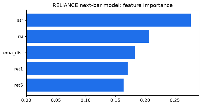
Treat this as a clue, not gospel - importance is measured on the training data and can itself be noisy. But a feature that the model consistently ignores across runs is a fair candidate for the bin.
Does it survive out-of-sample? Walk-forward for ML
A single train/test split can flatter you by luck. So we apply exactly the walk-forward discipline from Chapter 29, now to the model: retrain on a rolling window, grade on the next window, slide forward, repeat. We compare each window's accuracy to its own baseline. A model worth trading beats the baseline consistently, not just in one cherry-picked split.
# A walk-forward sanity check for ML: retrain each window, grade on the next.
import os
from datetime import datetime, timedelta

import pandas as pd
from openalgo import api, ta
from sklearn.ensemble import RandomForestClassifier
from sklearn.metrics import accuracy_score

client = api(
    api_key=os.getenv("OPENALGO_API_KEY", "your_api_key_here"),
    host=os.getenv("OPENALGO_HOST", "http://127.0.0.1:5000"),
)

end = datetime.now().strftime("%Y-%m-%d")
start = (datetime.now() - timedelta(days=900)).strftime("%Y-%m-%d")
df = client.history(symbol="RELIANCE", exchange="NSE", interval="D", start_date=start, end_date=end)
c = df["close"]
d = pd.DataFrame(index=df.index)
d["rsi"] = ta.rsi(c, 14); d["ret1"] = c.pct_change(); d["ret5"] = c.pct_change(5)
d["atr"] = ta.atr(df["high"], df["low"], c, 14); d["ema_dist"] = (c - ta.ema(c, 20)) / c
d["target"] = (c.shift(-1) > c).astype(int)
d = d.dropna()
X, y = d.drop(columns="target"), d["target"]

train_len, test_len, i, scores = 300, 100, 0, []
while i + train_len + test_len <= len(X):
    model = RandomForestClassifier(n_estimators=100, max_depth=4, random_state=0)
    model.fit(X.iloc[i:i + train_len], y.iloc[i:i + train_len])         # train on window
    te_X = X.iloc[i + train_len:i + train_len + test_len]
    te_y = y.iloc[i + train_len:i + train_len + test_len]
    acc = accuracy_score(te_y, model.predict(te_X))                     # grade next window
    base = max(te_y.mean(), 1 - te_y.mean())
    scores.append(acc)
    print(f"window {i // test_len + 1}: accuracy {acc:.1%}  vs baseline {base:.1%}")
    i += test_len
print(f"\nAverage out-of-sample accuracy: {sum(scores) / len(scores):.1%}")
print("Consistently beating the baseline across windows is the bar for a real edge.")window 1: accuracy 49.0% vs baseline 51.0% window 2: accuracy 50.0% vs baseline 50.0% Average out-of-sample accuracy: 49.5% Consistently beating the baseline across windows is the bar for a real edge.
If your model only beats the baseline in one window out of four, you don't have an edge - you have variance. This honest, unglamorous check is what separates a research toy from something you'd risk capital on.
The capstone: a complete trading bot
Everything now comes together in one script - the bot we promised on page one of this series. It does the full loop end to end: fetch history, engineer features and label, train a model, predict today's direction, place an order (safely, in analyze mode), and optionally send a Telegram alert. It's long-only: it enters on an up-signal and squares off to flat otherwise, using placesmartorder with a target position_size=0 - a clean, common pattern for a one-position bot.
# CAPSTONE: an end-to-end ML bot -- fetch, learn, signal, order (analyze), alert.
import os
from datetime import datetime, timedelta

import pandas as pd
from openalgo import api, ta
from sklearn.ensemble import RandomForestClassifier

client = api(
    api_key=os.getenv("OPENALGO_API_KEY", "your_api_key_here"),
    host=os.getenv("OPENALGO_HOST", "http://127.0.0.1:5000"),
)
SYMBOL, EXCHANGE = "RELIANCE", "NSE"

# 1) FETCH
end = datetime.now().strftime("%Y-%m-%d")
start = (datetime.now() - timedelta(days=900)).strftime("%Y-%m-%d")
df = client.history(symbol=SYMBOL, exchange=EXCHANGE, interval="D", start_date=start, end_date=end)
c = df["close"]
# 2) FEATURES + label (predict next bar up/down)
d = pd.DataFrame(index=df.index)
d["rsi"] = ta.rsi(c, 14); d["ret1"] = c.pct_change(); d["ema_dist"] = (c - ta.ema(c, 20)) / c
d["target"] = (c.shift(-1) > c).astype(int)
feats = ["rsi", "ret1", "ema_dist"]
train = d.dropna()                                            # rows with a known answer
# 3) TRAIN on all complete rows, then predict TODAY's row (whose answer is unknown)
model = RandomForestClassifier(n_estimators=120, max_depth=4, random_state=0)
model.fit(train[feats], train["target"])
today = d[feats].iloc[[-1]]                                   # latest features
signal = int(model.predict(today)[0])                         # 1 = expect up, 0 = expect down
print(f"Model signal for {SYMBOL}: predicted next bar {'UP' if signal else 'DOWN'}")

# 4) ACT -- long-only bot: enter on UP, square off to flat on DOWN. Safe in analyze mode.
if signal == 1:
    resp = client.placeorder(strategy="MLBot", symbol=SYMBOL, action="BUY",
                             exchange=EXCHANGE, price_type="MARKET", product="CNC", quantity=1)
    print("Enter long  ->", resp.get("status"), resp.get("orderid", resp.get("message")))
else:
    # placesmartorder with position_size=0 means "hold zero" -- it exits any long, else no-op.
    resp = client.placesmartorder(strategy="MLBot", symbol=SYMBOL, action="SELL",
                                  exchange=EXCHANGE, price_type="MARKET", product="CNC",
                                  quantity=0, position_size=0)
    print("Square off  ->", resp.get("status"), resp.get("message", resp.get("orderid")))
# 5) ALERT (optional) -- degrades gracefully if Telegram is not linked
try:
    alert = client.telegram(username=os.getenv("OPENALGO_TG_USER", "openalgo"),
                            message=f"MLBot {SYMBOL}: {'BUY' if signal else 'FLAT'}")
    print("Telegram:", alert.get("status"))
except Exception as exc:                                      # noqa: BLE001
print("Telegram skipped:", exc)Model signal for RELIANCE: predicted next bar DOWN Square off -> success No OpenPosition Found. Not placing Exit order. Telegram: error
The Telegram step uses client.telegram(username=..., message=...). It's wrapped in try/except so the bot keeps running even if Telegram isn't linked on your server - exactly the defensive habit from Chapter 2. Link your account from the OpenAlgo dashboard's Telegram page to receive live alerts, and your bot can ping your phone the moment it acts.
This runs in analyze mode, so every order is simulated. Before you ever flip to live, re-read the walk-forward results, confirm the edge is real, start with tiny size, and keep a human watching. A model is a tool, not a guarantee - and the market does not care how clever your neural network is.
Scheduling it. A bot that runs once is a script; a bot that runs every day is a system. To trade this daily, you schedule it to run a few minutes after the close (when the day's candle is final) - or near the open if you act on the prior day's signal. On Linux you'd use cron; on Windows, Task Scheduler; or you can paste the script straight into OpenAlgo's built-in Python strategy host and let it run on an IST schedule with live logs. Whatever the scheduler, the script itself stays exactly as you see it here.
Try it yourself
- Add two features to the capstone - say a 10-day RSI and
c.pct_change(10)- and re-run the walk-forward check. Does out-of-sample accuracy improve, or does the extra complexity just add noise? - Shrink the neural net to
hidden_layer_sizes=(4,)and grow it to(64, 32). Which generalises better out-of-sample? Let the result surprise you. - Point the capstone at an NFO future like
NIFTY30JUN26FUT(exchangeNFO) and adjust the product toNRML. Does the model read an index future differently from a single stock?
Recap
- A model learns rules from labelled examples; features are your numeric clues, and feature engineering matters more than the model choice.
- The label here is next-bar direction; always compare accuracy to the base rate, because beating it is the only thing that counts.
- Split with
shuffle=Falseso you train on the past and test on the future - never let the model peek ahead. - Logistic regression and random forests are sane baselines; the MLPClassifier is the neural network, and bigger networks overfit faster.
- Feature importance hints at what's predictive; a walk-forward check confirms whether any edge survives out-of-sample.
- The capstone bot fetches, learns, signals, orders in analyze mode, and alerts - then you schedule it with cron, Task Scheduler, or OpenAlgo's strategy host.
That's the series. You started by confirming an SDK was installed; you finish with a complete, machine-learning trading bot you understand line by line. The tools are now yours - use them honestly, test everything out-of-sample, respect the market's difficulty, and trade the edges you can actually prove.