Performance Metrics & Reporting
Sharpe, Sortino, CAGR, drawdown and win-rate - plus a full QuantStats report.
- ·CAGR & total return
- ·Sharpe & Sortino
- ·Max drawdown
- ·Win rate & profit factor
- ·Benchmark vs index
- ·QuantStats tearsheet
Your backtest spat out an equity curve and a wall of numbers. Now comes the judgement: is this strategy actually any good? "It made money" is not an answer - money made recklessly, with stomach-churning drawdowns, by getting lucky once, is not an edge. This chapter is about reading a strategy honestly, the way a professional risk manager would, and knowing what "good" looks like for each metric.
We'll take each headline number in turn - total return, CAGR, Sharpe, Sortino, max drawdown, win rate, profit factor - explain why it matters and what a healthy value looks like, compute it both from VectorBT and (once) by hand so there's no mystery, benchmark the strategy against the NIFTY index, and finish with a full QuantStats report you can save and share. Everything here uses NSE data and our familiar EMA-crossover strategy.
Don't be alarmed if some metrics in the live outputs are negative. A single strategy over one window can easily underperform - that's exactly why we measure. The skill we're building is reading the numbers honestly, not cherry-picking a flattering run.
Total return vs CAGR
Total return is the whole-period profit: turn ₹100,000 into ₹110,000 and that's +10%. Simple, but it hides time. A 40% gain is spectacular in one year and mediocre over five. CAGR (Compound Annual Growth Rate) fixes that by re-expressing the profit as a smooth yearly growth rate, so you can fairly compare backtests of different lengths. CAGR is the number you quote when someone asks "what does this return per year?"
# Total return vs CAGR: the same profit, told two different ways.
import datetime
import os

import vectorbt as vbt
from openalgo import api, ta

client = api(
    api_key=os.getenv("OPENALGO_API_KEY", "your_api_key_here"),
    host=os.getenv("OPENALGO_HOST", "http://127.0.0.1:5000"),
)

end = datetime.date.today()
start = end - datetime.timedelta(days=400)
df = client.history(symbol="RELIANCE", exchange="NSE", interval="D",
                    start_date=str(start), end_date=str(end))
close = df["close"].astype(float)
fast, slow = ta.ema(close, 10), ta.ema(close, 30)
entries = (fast > slow) & (fast.shift(1) <= slow.shift(1))
exits = (fast < slow) & (fast.shift(1) >= slow.shift(1))
pf = vbt.Portfolio.from_signals(close, entries, exits,
                                init_cash=100000, fees=0.001, slippage=0.0005, freq="1D")

# Total return = the whole-period profit. CAGR = that profit re-expressed as a
# smooth yearly growth rate, so you can compare tests of different lengths.
print(f"Total return: {pf.total_return() * 100:.2f}%  (over the whole test)")
print(f"CAGR        : {pf.annualized_return() * 100:.2f}%  (per year, compounded)")
print("CAGR is the fairer yardstick: a 40% gain in 4 years is far worse than in 1.")Total return: -7.24% (over the whole test) CAGR : -9.57% (per year, compounded) CAGR is the fairer yardstick: a 40% gain in 4 years is far worse than in 1.
Always compare strategies on CAGR, not total return, unless they cover the exact same period. Total return rewards a test simply for being longer; CAGR puts everything on a per-year footing.
Sharpe and Sortino: return per unit of risk
Return alone is half the story - you have to ask how much risk you took to get it. The Sharpe ratio divides your return by its volatility (the standard deviation of returns). It answers: "how much reward did I earn per unit of bumpiness?" Two strategies returning 15% are not equal if one rode a roller-coaster to get there.
The Sortino ratio is Sharpe's smarter cousin. It only counts downside volatility - the bad days. After all, no trader complains about an unusually big up day, yet plain Sharpe penalises it as "risk." Sortino measures the volatility that actually hurts.
# Sharpe and Sortino: return per unit of RISK, not return alone.
import datetime
import os

import vectorbt as vbt
from openalgo import api, ta

client = api(
    api_key=os.getenv("OPENALGO_API_KEY", "your_api_key_here"),
    host=os.getenv("OPENALGO_HOST", "http://127.0.0.1:5000"),
)

end = datetime.date.today()
start = end - datetime.timedelta(days=400)
df = client.history(symbol="RELIANCE", exchange="NSE", interval="D",
                    start_date=str(start), end_date=str(end))
close = df["close"].astype(float)
fast, slow = ta.ema(close, 10), ta.ema(close, 30)
entries = (fast > slow) & (fast.shift(1) <= slow.shift(1))
exits = (fast < slow) & (fast.shift(1) >= slow.shift(1))
pf = vbt.Portfolio.from_signals(close, entries, exits,
                                init_cash=100000, fees=0.001, slippage=0.0005, freq="1D")

# Sharpe divides return by ALL volatility. Sortino only counts DOWNSIDE
# volatility - it doesn't punish you for big up days, which traders prefer.
print(f"Sharpe ratio : {pf.sharpe_ratio():.2f}")
print(f"Sortino ratio: {pf.sortino_ratio():.2f}")
print("Rough guide: Sharpe above 1 is good, above 2 is excellent, "
"below 0 means you lost money.")Sharpe ratio : -0.66 Sortino ratio: -0.88 Rough guide: Sharpe above 1 is good, above 2 is excellent, below 0 means you lost money.
A rough rule of thumb for an annualised Sharpe: below 0 means you lost money, around 1 is good, 2 is excellent, 3+ is suspiciously good (check for look-ahead bias or overfitting). Sortino is usually a touch higher than Sharpe for the same strategy, because it ignores upside swings.
Max drawdown: the pain you must survive
This is the metric that decides whether you can actually trade a strategy without abandoning it. Maximum drawdown is the worst peak-to-trough fall your equity ever suffered - measured from the highest point it had reached. A 50% drawdown isn't just "down 50%": you then need a 100% gain just to get back to even. Deep drawdowns end accounts and break nerve, regardless of the final return.
The Calmar ratio pairs the two ideas - CAGR divided by max drawdown - to ask "how much annual return did I earn per unit of worst-case pain?"
# Max drawdown: the worst peak-to-trough fall - the pain you must stomach.
import datetime
import os

import vectorbt as vbt
from openalgo import api, ta

client = api(
    api_key=os.getenv("OPENALGO_API_KEY", "your_api_key_here"),
    host=os.getenv("OPENALGO_HOST", "http://127.0.0.1:5000"),
)

end = datetime.date.today()
start = end - datetime.timedelta(days=400)
df = client.history(symbol="RELIANCE", exchange="NSE", interval="D",
                    start_date=str(start), end_date=str(end))
close = df["close"].astype(float)
fast, slow = ta.ema(close, 10), ta.ema(close, 30)
entries = (fast > slow) & (fast.shift(1) <= slow.shift(1))
exits = (fast < slow) & (fast.shift(1) >= slow.shift(1))
pf = vbt.Portfolio.from_signals(close, entries, exits,
                                init_cash=100000, fees=0.001, slippage=0.0005, freq="1D")

# Drawdown is measured from the highest equity peak so far. The max is the
# deepest valley - the loss you'd have lived through at the worst moment.
print(f"Max drawdown : {pf.max_drawdown() * 100:.2f}%")
print(f"Calmar ratio : {pf.calmar_ratio():.2f}  (CAGR divided by max drawdown)")
print("A 50% drawdown needs a 100% gain just to recover - shallow is survivable, "
"deep can end an account.")Max drawdown : -13.80% Calmar ratio : -0.69 (CAGR divided by max drawdown) A 50% drawdown needs a 100% gain just to recover - shallow is survivable, deep can end an account.
A backtest can show a fat total return and still be untradeable. If the path there included a 60% drawdown, almost no human would have held on through it. Judge a strategy by the worst night it would have given you, not just the destination.
Win rate and profit factor
Now we look inside the trades. Win rate is the percentage of trades that made money. It feels like the headline number - but on its own it's a trap. Profit factor is the truth-teller: gross profit divided by gross loss. Above 1 means your winners outweigh your losers in rupees. A trend-following system often wins less than half its trades yet is highly profitable, because the rare big winners dwarf the many small losses it cuts quickly.
# Win rate and profit factor: how OFTEN you win vs how MUCH you win.
import datetime
import os

import vectorbt as vbt
from openalgo import api, ta

client = api(
    api_key=os.getenv("OPENALGO_API_KEY", "your_api_key_here"),
    host=os.getenv("OPENALGO_HOST", "http://127.0.0.1:5000"),
)

end = datetime.date.today()
start = end - datetime.timedelta(days=400)
df = client.history(symbol="RELIANCE", exchange="NSE", interval="D",
                    start_date=str(start), end_date=str(end))
close = df["close"].astype(float)
fast, slow = ta.ema(close, 10), ta.ema(close, 30)
entries = (fast > slow) & (fast.shift(1) <= slow.shift(1))
exits = (fast < slow) & (fast.shift(1) >= slow.shift(1))
pf = vbt.Portfolio.from_signals(close, entries, exits,
                                init_cash=100000, fees=0.001, slippage=0.0005, freq="1D")
trades = pf.trades

# Profit factor = gross profit / gross loss. Above 1 means the wins outweigh
# the losses. A trend system often wins LESS than half its trades yet still
# profits, because the few wins are far bigger than the many small losses.
print(f"Total trades : {trades.count()}")
print(f"Win rate     : {trades.win_rate() * 100:.1f}%")
print(f"Profit factor: {trades.profit_factor():.2f}  (>1 = profitable)")
print("Don't chase a high win rate alone - many tiny wins can be wiped by one big loss.")Total trades : 4 Win rate : 25.0% Profit factor: 0.32 (>1 = profitable) Don't chase a high win rate alone - many tiny wins can be wiped by one big loss.
Never judge a strategy by win rate alone. A 90% win rate with one catastrophic loser can still blow up your account; a 35% win rate with disciplined, large winners can compound beautifully. Profit factor > 1 is the real bar to clear.
There's no magic - compute them yourself
To prove these metrics aren't sorcery, let's compute Sharpe and CAGR straight from a returns series with a few lines of NumPy, and check them against VectorBT's. Sharpe is just mean / std * sqrt(252) (annualising daily numbers by the ~252 trading days in a year); CAGR comes from compounding the daily returns. The values land in the same ballpark - small gaps are just library conventions - and the point is made: you understand what's under the hood.
# The same metrics computed by hand from a daily-returns series - no magic.
import datetime
import os

import numpy as np
import vectorbt as vbt
from openalgo import api, ta

client = api(
    api_key=os.getenv("OPENALGO_API_KEY", "your_api_key_here"),
    host=os.getenv("OPENALGO_HOST", "http://127.0.0.1:5000"),
)

end = datetime.date.today()
start = end - datetime.timedelta(days=400)
df = client.history(symbol="INFY", exchange="NSE", interval="D",
                    start_date=str(start), end_date=str(end))
close = df["close"].astype(float)
fast, slow = ta.ema(close, 10), ta.ema(close, 30)
entries = (fast > slow) & (fast.shift(1) <= slow.shift(1))
exits = (fast < slow) & (fast.shift(1) >= slow.shift(1))
pf = vbt.Portfolio.from_signals(close, entries, exits,
                                init_cash=100000, fees=0.001, slippage=0.0005, freq="1D")

rets = pf.returns()                       # daily strategy returns
# Sharpe = mean / std of daily returns, scaled to a year (252 trading days).
sharpe = rets.mean() / rets.std() * np.sqrt(252)
# CAGR from compounding the daily returns.
total_growth = (1 + rets).prod()
cagr = total_growth ** (252 / len(rets)) - 1
print(f"Hand Sharpe : {sharpe:.2f}   vs VectorBT {pf.sharpe_ratio():.2f}")
print(f"Hand CAGR   : {cagr * 100:.2f}%  vs VectorBT {pf.annualized_return() * 100:.2f}%")
print("Same ballpark - small gaps come from library conventions (how open trades")
print("and the exact day-count are handled). The point: there is no magic here.")Hand Sharpe : -0.61 vs VectorBT -0.73 Hand CAGR : -9.58% vs VectorBT -13.57% Same ballpark - small gaps come from library conventions (how open trades and the exact day-count are handled). The point: there is no magic here.
Benchmark against the index
Here's the question that humbles most strategies: did you beat simply holding the market? A 12% return sounds great until you learn the NIFTY index returned 20% over the same window with zero effort and no single-stock risk. Your strategy's job is to add value over that free alternative. We hold the NIFTY index (on the NSE_INDEX exchange) as our benchmark and measure the edge.
# A return is only impressive next to a benchmark: beat NIFTY buy-and-hold?
import datetime
import os

import vectorbt as vbt
from openalgo import api, ta

client = api(
    api_key=os.getenv("OPENALGO_API_KEY", "your_api_key_here"),
    host=os.getenv("OPENALGO_HOST", "http://127.0.0.1:5000"),
)

end = datetime.date.today()
start = end - datetime.timedelta(days=400)
df = client.history(symbol="RELIANCE", exchange="NSE", interval="D",
                    start_date=str(start), end_date=str(end))
close = df["close"].astype(float)
fast, slow = ta.ema(close, 10), ta.ema(close, 30)
entries = (fast > slow) & (fast.shift(1) <= slow.shift(1))
exits = (fast < slow) & (fast.shift(1) >= slow.shift(1))
pf = vbt.Portfolio.from_signals(close, entries, exits,
                                init_cash=100000, fees=0.001, slippage=0.0005, freq="1D")

# Benchmark: just hold the NIFTY index over the same window. Indices live on
# the NSE_INDEX exchange.
nifty = client.history(symbol="NIFTY", exchange="NSE_INDEX", interval="D",
                       start_date=str(start), end_date=str(end))
nifty_close = nifty["close"].astype(float)
nifty_return = (nifty_close.iloc[-1] / nifty_close.iloc[0] - 1) * 100

print(f"Strategy return : {pf.total_return() * 100:.2f}%")
print(f"NIFTY buy & hold: {nifty_return:.2f}%")
edge = pf.total_return() * 100 - nifty_return
print(f"Edge over index : {edge:+.2f}% ({'beat' if edge > 0 else 'lagged'} the market)")Strategy return : -7.24% NIFTY buy & hold: -4.61% Edge over index : -2.63% (lagged the market)
The index is the honest yardstick. If your active, trade-every-week strategy can't beat a buy-and-hold of NIFTY after costs, the rational move is to just hold the index. Beating the benchmark - ideally with less drawdown - is what justifies all the work.
QuantStats: a full report in one line
Computing metrics one by one is great for learning; for everyday work, QuantStats does it all from a single returns series. qs.stats.sharpe(returns), qs.stats.sortino(...), qs.stats.max_drawdown(...), qs.stats.cagr(...) each return one clean number.
# QuantStats gives the same metrics straight from a returns series, in one import.
import datetime
import os

import quantstats as qs
import vectorbt as vbt
from openalgo import api, ta

client = api(
    api_key=os.getenv("OPENALGO_API_KEY", "your_api_key_here"),
    host=os.getenv("OPENALGO_HOST", "http://127.0.0.1:5000"),
)

end = datetime.date.today()
start = end - datetime.timedelta(days=400)
df = client.history(symbol="HDFCBANK", exchange="NSE", interval="D",
                    start_date=str(start), end_date=str(end))
close = df["close"].astype(float)
fast, slow = ta.ema(close, 10), ta.ema(close, 30)
entries = (fast > slow) & (fast.shift(1) <= slow.shift(1))
exits = (fast < slow) & (fast.shift(1) >= slow.shift(1))
pf = vbt.Portfolio.from_signals(close, entries, exits,
                                init_cash=100000, fees=0.001, slippage=0.0005, freq="1D")

# qs.stats.* takes a pandas Series of returns and returns one number each.
rets = pf.returns()
print(f"Sharpe      : {qs.stats.sharpe(rets):.2f}")
print(f"Sortino     : {qs.stats.sortino(rets):.2f}")
print(f"Max drawdown: {qs.stats.max_drawdown(rets) * 100:.2f}%")
print(f"CAGR        : {qs.stats.cagr(rets) * 100:.2f}%")
print(f"Volatility : {qs.stats.volatility(rets) * 100:.2f}% (annualised)")Sharpe : -0.90 Sortino : -1.19 Max drawdown: -9.75% CAGR : -7.50% Volatility : 8.31% (annualised)
And qs.reports.metrics(...) produces a complete tearsheet-style table - your strategy beside the benchmark across dozens of metrics. We pass display=False to get it back as a tidy DataFrame, print the headline rows, and save the full table to a text file you can keep alongside your results.
# A full QuantStats metrics report - strategy vs NIFTY - saved to a text file.
import datetime
import os
import sys
from pathlib import Path

try:
    sys.stdout.reconfigure(encoding="utf-8")   # report uses a few unicode symbols
except Exception:
    pass

import quantstats as qs
import vectorbt as vbt
from openalgo import api, ta

client = api(
    api_key=os.getenv("OPENALGO_API_KEY", "your_api_key_here"),
    host=os.getenv("OPENALGO_HOST", "http://127.0.0.1:5000"),
)

end = datetime.date.today()
start = end - datetime.timedelta(days=400)
df = client.history(symbol="ICICIBANK", exchange="NSE", interval="D",
                    start_date=str(start), end_date=str(end))
close = df["close"].astype(float)
fast, slow = ta.ema(close, 10), ta.ema(close, 30)
entries = (fast > slow) & (fast.shift(1) <= slow.shift(1))
exits = (fast < slow) & (fast.shift(1) >= slow.shift(1))
pf = vbt.Portfolio.from_signals(close, entries, exits,
                                init_cash=100000, fees=0.001, slippage=0.0005, freq="1D")
rets = pf.returns()
nifty = client.history(symbol="NIFTY", exchange="NSE_INDEX", interval="D",
                       start_date=str(start), end_date=str(end))
bench = nifty["close"].astype(float).pct_change().fillna(0).reindex(rets.index).fillna(0)

# display=False returns a tidy DataFrame (Strategy vs Benchmark) we can print/save.
report = qs.reports.metrics(rets, benchmark=bench, mode="basic", display=False)
report.index = [str(i).replace("﹪", "%") for i in report.index]   # tidy labels

# Print a curated set of headline rows (Strategy column) for a quick read.
for row in ["Cumulative Return", "CAGR%", "Sharpe", "Sortino",
            "Max Drawdown", "Win Rate", "Profit Factor"]:
    if row in report.index:
        print(f"{row:18s}: {report.loc[row, 'Strategy']}")

# Save the FULL strategy-vs-benchmark table to a UTF-8 text file.
out = Path(__file__).with_name("metrics_report.txt")
out.write_text(report.to_string(), encoding="utf-8")
print(f"\nFull strategy-vs-NIFTY report saved to {out.name}")Cumulative Return : -0.24 CAGR% : -0.23 Sharpe : -2.82 Sortino : -3.26 Max Drawdown : - Profit Factor : 0.43 Full strategy-vs-NIFTY report saved to metrics_report.txt
QuantStats prints a couple of special symbols (like the % in CAGR%) that can upset a plain Windows console. Two safe habits: add sys.stdout.reconfigure(encoding="utf-8") at the top of the script, and save the report to a UTF-8 text file with display=False rather than relying on screen printing.
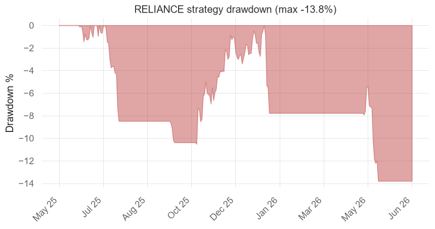
A picture of the pain
Finally, a chart that says more than any single number: the drawdown curve. It shades how far below its running peak the equity sat, every day of the test - so you can see not just how deep the worst fall was, but how long you'd have spent underwater waiting to recover. We save it as a PNG.
# Plot the drawdown curve - a picture of how deep and how long the pain lasted.
import datetime
import os
from pathlib import Path

import matplotlib

matplotlib.use("Agg")
import matplotlib.pyplot as plt
import vectorbt as vbt
from openalgo import api, ta

client = api(
    api_key=os.getenv("OPENALGO_API_KEY", "your_api_key_here"),
    host=os.getenv("OPENALGO_HOST", "http://127.0.0.1:5000"),
)

end = datetime.date.today()
start = end - datetime.timedelta(days=400)
df = client.history(symbol="RELIANCE", exchange="NSE", interval="D",
                    start_date=str(start), end_date=str(end))
close = df["close"].astype(float)
fast, slow = ta.ema(close, 10), ta.ema(close, 30)
entries = (fast > slow) & (fast.shift(1) <= slow.shift(1))
exits = (fast < slow) & (fast.shift(1) >= slow.shift(1))
pf = vbt.Portfolio.from_signals(close, entries, exits,
                                init_cash=100000, fees=0.001, slippage=0.0005, freq="1D")

# Drawdown = how far below the running peak the equity sits, as a percentage.
equity = pf.value()
drawdown = (equity / equity.cummax() - 1) * 100
x = list(range(len(drawdown)))                        # positional x, no gaps
fig, ax = plt.subplots(figsize=(9, 4))
ax.fill_between(x, drawdown.values, 0, color="firebrick", alpha=0.4)
ax.set_title(f"RELIANCE strategy drawdown (max {drawdown.min():.1f}%)")
ax.set_ylabel("Drawdown %")
step = max(1, len(drawdown) // 8)
ax.set_xticks(x[::step])
ax.set_xticklabels(drawdown.index[::step].strftime("%b %y"), rotation=45, ha="right")
out = Path(__file__).with_suffix(".png")
fig.savefig(out, dpi=110, bbox_inches="tight")
print(f"Worst drawdown: {drawdown.min():.2f}%")
print(f"Saved {out.name}")Worst drawdown: -13.80% Saved 09_drawdown_png.png
Try it yourself
- Run the benchmark example for three different stocks. How many of them actually beat NIFTY?
- In the win-rate example, note the win rate and profit factor together - is it a "few big winners" strategy or a "many small winners" one?
- Open the saved
metrics_report.txtand find the Sharpe, Sortino and max-drawdown rows for both the strategy and the benchmark. Which one would you actually trade?
Recap
- Total return ignores time; CAGR is the fair per-year yardstick for comparing tests.
- Sharpe is return per unit of all volatility; Sortino counts only the downside that actually hurts. Above 1 is good, above 2 excellent.
- Max drawdown is the worst peak-to-trough fall and decides whether you could survive the strategy; Calmar pairs it with CAGR.
- Win rate alone is a trap - profit factor > 1 (and the size of winners vs losers) is what proves an edge.
- Always benchmark against the index: beating a free buy-and-hold of NIFTY, with less pain, is the whole point.
- QuantStats turns a returns series into individual metrics and a full report - save it to UTF-8 to avoid console encoding errors.
You can now place orders, prove an edge, and judge it honestly. From here the series moves into making strategies robust - optimising parameters without overfitting, then walk-forward testing - before we hand the keys to a machine-learning model and wire up a complete bot.