Seasonal & Calendar Strategies
Day-of-week, month and expiry-week effects measured straight from history.
- ·Day-of-week returns
- ·Monthly seasonality
- ·Turn-of-month effect
- ·Expiry-week behaviour
- ·Calendar masks in Pandas
- ·Backtest a seasonal rule
Every trader has heard the market folklore. "Sell in May." "Markets are weak on expiry day." "Stocks drift up around month-end when salary money flows in." These are claims about seasonality - the idea that the calendar itself, the plain fact of which day or month it is, nudges returns one way or another. The trouble is that folklore is cheap and memory is unreliable. You remember the three Mondays that crashed and forget the thirty that didn't.
This chapter is about settling those arguments with data instead of opinion. We'll take years of history and ask precise, testable questions: Is Wednesday really stronger than Tuesday? Is April genuinely the best month? Do the last days of the month behave differently from the middle? Pandas makes this almost embarrassingly easy - a single groupby answers most of them. And once we can measure an effect, we'll do the honest thing and backtest a rule built on it, to see whether the edge survives contact with reality.
A gentle warning before we start: seasonal effects are real but small and noisy. They are a tilt, not a crystal ball. Treat what follows as a way to study the market's habits, not as a guaranteed money machine.
Everything here is ordinary Pandas on a price DataFrame - the same client.history() call and the same rolling/groupby tools from Chapters 5 and 7. If those felt comfortable, this chapter is mostly new questions, not new tools. We'll use the NIFTY index throughout because it has a long, clean history and is the reference for Indian F&O.
The raw material: history and daily returns
Seasonality is measured on returns, not prices. A price of 24,000 tells you nothing about a Tuesday; a return of +0.4% does. So every example in this chapter starts the same way: pull a long stretch of daily candles, then add a daily return column - today's close compared with yesterday's, as a percentage. In Pandas that is one method, .pct_change().
We ask for roughly 900 calendar days of history (about two and a half years of trading) so that each weekday and month has enough samples to mean something.
# Foundation: pull years of NIFTY daily candles and add a daily-return column.
import os
from datetime import datetime, timedelta

from openalgo import api

client = api(
    api_key=os.getenv("OPENALGO_API_KEY", "your_api_key_here"),
    host=os.getenv("OPENALGO_HOST", "http://127.0.0.1:5000"),
)

end = datetime.now().strftime("%Y-%m-%d")
start = (datetime.now() - timedelta(days=900)).strftime("%Y-%m-%d")

df = client.history(symbol="NIFTY", exchange="NSE_INDEX", interval="D", start_date=start, end_date=end)

# Daily return = today's close vs yesterday's close, as a percentage.
df["ret"] = df["close"].pct_change() * 100

print("Trading days loaded:", len(df))
print("Date range:", df.index.min().date(), "to", df.index.max().date())
print("\nLast 3 days with returns:")
print(df[["close", "ret"]].tail(3).round(2))Trading days loaded: 610
Date range: 2024-01-05 to 2026-06-23
Last 3 days with returns:
close ret
timestamp
2026-06-19 24013.10 -0.64
2026-06-22 24102.90 0.37
2026-06-23 23795.25 -1.28pct_change() computes (today - yesterday) / yesterday. Multiplying by 100 turns it into a percentage. The very first row has no "yesterday", so it comes out as NaN (Not a Number) - that's normal, and we either drop it or fill it with 0 before doing maths on the column.
Day-of-week effects
Here is the first real question. Pandas indexes our DataFrame by timestamp, and that index knows what day of the week each row is: df.index.dayofweek gives 0 for Monday through 4 for Friday. If we group the returns by that number and take the average of each group, we get the historical average return for every weekday - the whole "is Monday weak?" debate answered in three lines.
groupby is the workhorse here. Read df.groupby(df.index.dayofweek)["ret"].mean() as: "split the returns into buckets by weekday, then average each bucket."
# Day-of-week seasonality: which weekday has historically paid the most?
import os
from datetime import datetime, timedelta

from openalgo import api

client = api(
    api_key=os.getenv("OPENALGO_API_KEY", "your_api_key_here"),
    host=os.getenv("OPENALGO_HOST", "http://127.0.0.1:5000"),
)

end = datetime.now().strftime("%Y-%m-%d")
start = (datetime.now() - timedelta(days=900)).strftime("%Y-%m-%d")
df = client.history(symbol="NIFTY", exchange="NSE_INDEX", interval="D", start_date=start, end_date=end)

df["ret"] = df["close"].pct_change() * 100
df = df.dropna(subset=["ret"])
# index.dayofweek: Monday=0 ... Friday=4. Keep regular weekdays, group, average.
df = df[df.index.dayofweek < 5]
names = {0: "Mon", 1: "Tue", 2: "Wed", 3: "Thu", 4: "Fri"}
by_day = df.groupby(df.index.dayofweek)["ret"].agg(["mean", "count"])
by_day.index = by_day.index.map(names)

print("Average NIFTY return by weekday (%):")
print(by_day.round(3))
print("\nBest weekday on average:", by_day["mean"].idxmax())Average NIFTY return by weekday (%):
mean count
timestamp
Mon 0.040 122
Tue -0.064 126
Wed 0.189 118
Thu -0.007 119
Fri -0.041 119
Best weekday on average: WedNotice we also print a count for each weekday. That matters: an eye-catching average built on only a handful of days is noise dressed as signal. A difference backed by 120 Wednesdays is far more trustworthy than one backed by 12.
A weekday being "best on average" in the past is not a promise about next Wednesday. These averages are tiny - often a few hundredths of a percent - and they wobble if you change the date window. Always sanity-check how stable an effect is before you trade it.
Month-of-year seasonality
The same idea scales up to months. But here we don't want to average daily returns - we want each calendar month's total return, then compare like with like across years. So we first resample the daily closes to month-end values ("ME" means "month end"), take the percentage change between consecutive month-ends, and finally group those monthly returns by their month number.
# Month-of-year seasonality: roll daily returns up into a return for each month.
import os
from datetime import datetime, timedelta

from openalgo import api

client = api(
    api_key=os.getenv("OPENALGO_API_KEY", "your_api_key_here"),
    host=os.getenv("OPENALGO_HOST", "http://127.0.0.1:5000"),
)

end = datetime.now().strftime("%Y-%m-%d")
start = (datetime.now() - timedelta(days=900)).strftime("%Y-%m-%d")
df = client.history(symbol="NIFTY", exchange="NSE_INDEX", interval="D", start_date=start, end_date=end)

# Resample to month-end and compute each calendar month's total return (%).
monthly = df["close"].resample("ME").last().pct_change() * 100
# Group those monthly returns by their month number (1..12) and average.
names = {1: "Jan", 2: "Feb", 3: "Mar", 4: "Apr", 5: "May", 6: "Jun",
         7: "Jul", 8: "Aug", 9: "Sep", 10: "Oct", 11: "Nov", 12: "Dec"}
by_month = monthly.groupby(monthly.index.month).mean()
by_month.index = by_month.index.map(names)

print("Average NIFTY return by calendar month (%):")
print(by_month.round(2))
print("\nHistorically strongest month:", by_month.idxmax())
print("Historically weakest month: ", by_month.idxmin())Average NIFTY return by calendar month (%): timestamp Jan -1.84 Feb -1.75 Mar -1.15 Apr 4.06 May -0.16 Jun 3.57 Jul 0.49 Aug -0.12 Sep 1.52 Oct -0.85 Nov 0.78 Dec -1.15 Name: close, dtype: float64 Historically strongest month: Apr Historically weakest month: Jan
The output is the classic seasonality table: a single average return for each of the twelve months. You'll often see a strong April (the start of the Indian financial year) and softer patches elsewhere. Whether that repeats is exactly the kind of thing you'd want to test before leaning on it.
The turn-of-month effect
One of the most studied calendar patterns is the turn of the month - the cluster of trading days spanning the last day or two of one month and the first few of the next. The theory is that institutional flows (salary credits, fund inflows, index rebalancing) bunch up there. To test it we need to rank each trading day within its own month.
Two small Pandas tricks do the job. index.to_period("M") collapses every date down to its month, giving us a grouping key. Then cumcount() numbers the rows inside each group - counting up from the start gives a day-of-month rank, and counting ascending=False tells us how far each day is from the month's end.
# Turn-of-month effect: are the last + first few trading days unusually strong?
import os
from datetime import datetime, timedelta

from openalgo import api

client = api(
    api_key=os.getenv("OPENALGO_API_KEY", "your_api_key_here"),
    host=os.getenv("OPENALGO_HOST", "http://127.0.0.1:5000"),
)

end = datetime.now().strftime("%Y-%m-%d")
start = (datetime.now() - timedelta(days=900)).strftime("%Y-%m-%d")
df = client.history(symbol="NIFTY", exchange="NSE_INDEX", interval="D", start_date=start, end_date=end)

df["ret"] = df["close"].pct_change() * 100
# Rank each trading day inside its own month: 1, 2, 3 ... from the start.
month_key = df.index.to_period("M")
df["dom_rank"] = df.groupby(month_key).cumcount() + 1          # day-of-month rank
df["from_end"] = df.groupby(month_key).cumcount(ascending=False)  # 0 = last day

# Turn-of-month window = last 2 days of a month OR first 3 days of the next.
tom = (df["from_end"] <= 1) | (df["dom_rank"] <= 3)

print("Turn-of-month days :", int(tom.sum()))
print("Other days         :", int((~tom).sum()))
print("Avg return on turn-of-month days (%):", round(df.loc[tom, "ret"].mean(), 3))
print("Avg return on all other days (%):", round(df.loc[~tom, "ret"].mean(), 3))Turn-of-month days : 150 Other days : 460 Avg return on turn-of-month days (%): -0.053 Avg return on all other days (%): 0.042
We then build a single condition - "last two days of a month OR first three of the next" - and compare the average return inside that window against everything else. If the turn-of-month days are meaningfully stronger, the folklore has some support.
Calendar masks: turning the calendar into a filter
So far we've grouped and averaged. The next step toward an actual strategy is the boolean mask - a column of True/False values, one per trading day, that says whether each day matches some calendar condition. df.index.dayofweek == 0 is a mask that's True on every Monday. df.index.month >= 10 is True in the last quarter.
The power comes from combining masks with & (and) and | (or), exactly the way you'd combine conditions in a trading rule. "Fridays in the last quarter" is just is_friday & is_q4. Once you have a mask, df.loc[mask, "ret"] pulls out only the returns on the matching days.
# Boolean calendar masks: a True/False filter you can AND/OR like a trading rule.
import os
from datetime import datetime, timedelta

from openalgo import api

client = api(
    api_key=os.getenv("OPENALGO_API_KEY", "your_api_key_here"),
    host=os.getenv("OPENALGO_HOST", "http://127.0.0.1:5000"),
)

end = datetime.now().strftime("%Y-%m-%d")
start = (datetime.now() - timedelta(days=900)).strftime("%Y-%m-%d")
df = client.history(symbol="NIFTY", exchange="NSE_INDEX", interval="D", start_date=start, end_date=end)

df["ret"] = df["close"].pct_change() * 100

# Each mask is a column of True/False, one per trading day.
is_monday = df.index.dayofweek == 0
is_friday = df.index.dayofweek == 4
is_q4 = df.index.month >= 10            # Oct, Nov, Dec

# Combine masks with & (and) / | (or) to express a precise calendar rule.
friday_in_q4 = is_friday & is_q4

print("Mondays in data :", int(is_monday.sum()), "| avg ret %:", round(df.loc[is_monday, "ret"].mean(), 3))
print("Fridays in data :", int(is_friday.sum()), "| avg ret %:", round(df.loc[is_friday, "ret"].mean(), 3))
print("Fridays in Q4 :", int(friday_in_q4.sum()), "| avg ret %:", round(df.loc[friday_in_q4, "ret"].mean(), 3))Mondays in data : 122 | avg ret %: 0.04 Fridays in data : 120 | avg ret %: -0.041 Fridays in Q4 : 25 | avg ret %: 0.101
A mask is the bridge between analysis and strategy. Every seasonal rule you will ever write boils down to: build a boolean mask describing "when am I allowed to be in the market", then apply it. Get comfortable creating and combining them - &, |, and ~ (not) are your verbs.
Expiry-week behaviour
For anyone trading index options or futures, the weekly expiry day has its own reputation - premiums decay, positions unwind, and price can behave oddly. NIFTY's weekly options currently expire on a Tuesday, but expiry weekdays have shifted over the years, so we do the professional thing and discover the expiry weekday at runtime from client.expiry() rather than hard-coding it. Then we compare returns on the expiry weekday against every other day.
# Expiry-week behaviour: discover the weekly expiry weekday, then test its returns.
import os
from datetime import datetime, timedelta

from openalgo import api

client = api(
    api_key=os.getenv("OPENALGO_API_KEY", "your_api_key_here"),
    host=os.getenv("OPENALGO_HOST", "http://127.0.0.1:5000"),
)

# Discover the weekday weekly options expire on -- never hard-code it.
expiries = client.expiry(symbol="NIFTY", exchange="NFO", instrumenttype="options")["data"]
near = [datetime.strptime(d, "%d-%b-%y") for d in expiries[:4]]
expiry_dow = max({d.weekday() for d in near}, key=[d.weekday() for d in near].count)
dow_name = ["Mon", "Tue", "Wed", "Thu", "Fri", "Sat", "Sun"][expiry_dow]
print("Weekly NIFTY options expire on:", dow_name, f"(weekday {expiry_dow})")

end = datetime.now().strftime("%Y-%m-%d")
start = (datetime.now() - timedelta(days=900)).strftime("%Y-%m-%d")
df = client.history(symbol="NIFTY", exchange="NSE_INDEX", interval="D", start_date=start, end_date=end)
df["ret"] = df["close"].pct_change() * 100

on_expiry = df.index.dayofweek == expiry_dow
print(f"\nAvg return on expiry day ({dow_name}) %:", round(df.loc[on_expiry, "ret"].mean(), 3))
print("Avg return on all other days       %:", round(df.loc[~on_expiry, "ret"].mean(), 3))
print("Expiry-day win rate %:", round((df.loc[on_expiry, "ret"] > 0).mean() * 100, 1))Weekly NIFTY options expire on: Tue (weekday 1) Avg return on expiry day (Tue) %: -0.064 Avg return on all other days %: 0.041 Expiry-day win rate %: 49.2
This pattern - ask the platform what the rules currently are, then measure - is one you'll reuse constantly. Hard-coded calendar facts rot; discovered ones don't.
Backtesting a seasonal rule
Measuring an effect is only half the job. The honest question is: if I had actually traded this, would I have done better than simply holding? So we build the simplest possible seasonal strategy - be long only on the weekdays that were historically positive, and sit in cash the rest of the time - and compare its growth against buy-and-hold.
The mechanics are a clean three-step recipe. First, learn which weekdays had a positive average return. Second, build a "strategy return" series that earns the day's return only when we're allowed to be in the market (and 0 otherwise). Third, compound both return series from a notional starting value of 100 using (1 + ret).cumprod(), which turns a stream of daily percentage moves into an equity curve.
# Backtest a seasonal rule: be long ONLY on historically strong weekdays.
import os
from datetime import datetime, timedelta

from openalgo import api

client = api(
    api_key=os.getenv("OPENALGO_API_KEY", "your_api_key_here"),
    host=os.getenv("OPENALGO_HOST", "http://127.0.0.1:5000"),
)

end = datetime.now().strftime("%Y-%m-%d")
start = (datetime.now() - timedelta(days=900)).strftime("%Y-%m-%d")
df = client.history(symbol="NIFTY", exchange="NSE_INDEX", interval="D", start_date=start, end_date=end)

df["ret"] = df["close"].pct_change().fillna(0)
# Step 1: learn which weekdays were positive on average.
strong = df.groupby(df.index.dayofweek)["ret"].mean()
strong_days = strong[strong > 0].index.tolist()
names = {0: "Mon", 1: "Tue", 2: "Wed", 3: "Thu", 4: "Fri"}
print("Strong weekdays (held):", [names[d] for d in strong_days])

# Step 2: the rule earns the day's return only when that weekday is "strong".
in_market = df.index.dayofweek.isin(strong_days)
df["strategy"] = df["ret"].where(in_market, 0.0)

# Step 3: compound both equity curves from a notional 100.
buy_hold = (1 + df["ret"]).cumprod() * 100
seasonal = (1 + df["strategy"]).cumprod() * 100
print("\nBuy & hold final value :", round(buy_hold.iloc[-1], 1))
print("Seasonal rule final    :", round(seasonal.iloc[-1], 1))
print("Days in market :", int(in_market.sum()), "of", len(df))Strong weekdays (held): ['Mon', 'Wed'] Buy & hold final value : 109.6 Seasonal rule final : 130.1 Days in market : 240 of 610
This backtest has a deliberate flaw worth naming: it picks the strong weekdays using the same data it then tests on. That's a mild form of look-ahead bias - using information you wouldn't have had in real time. The numbers look good partly because the rule was fitted to this exact history. In Chapters 26 and 29 we'll fix this properly with out-of-sample testing. For now, treat the result as a sketch of the idea, not proof of an edge.
Seeing it all at once
Tables are precise but a picture lands faster. A heatmap of monthly returns - years down the side, months across the top, green for gains and red for losses - lets you spot a seasonal pattern in a glance and, just as importantly, judge how consistent it is. A month that's green every year is far more convincing than one that averages green because of a single huge outlier.
# Visualise seasonality: a year x month grid of NIFTY monthly returns.
import os
from datetime import datetime, timedelta
from pathlib import Path

import matplotlib.pyplot as plt
from openalgo import api

client = api(
    api_key=os.getenv("OPENALGO_API_KEY", "your_api_key_here"),
    host=os.getenv("OPENALGO_HOST", "http://127.0.0.1:5000"),
)

end = datetime.now().strftime("%Y-%m-%d")
start = (datetime.now() - timedelta(days=1100)).strftime("%Y-%m-%d")
df = client.history(symbol="NIFTY", exchange="NSE_INDEX", interval="D", start_date=start, end_date=end)

monthly = df["close"].resample("ME").last().pct_change() * 100
grid = monthly.groupby([monthly.index.year, monthly.index.month]).mean().unstack()

fig, ax = plt.subplots(figsize=(9, 3.5))
im = ax.imshow(grid.values, cmap="RdYlGn", aspect="auto", vmin=-8, vmax=8)
ax.set_xticks(range(len(grid.columns)))
ax.set_xticklabels(["J", "F", "M", "A", "M", "J", "J", "A", "S", "O", "N", "D"][:len(grid.columns)])
ax.set_yticks(range(len(grid.index)))
ax.set_yticklabels(grid.index)
ax.set_title("NIFTY monthly return (%) by year")
fig.colorbar(im, ax=ax, label="% return")

out = Path(__file__).with_suffix(".png")
plt.savefig(out, dpi=110, bbox_inches="tight")
print("Saved", out.name)
print(grid.round(1))Saved 08_monthly_heatmap.png timestamp 1 2 3 4 5 6 7 8 9 10 11 12 timestamp 2023 NaN NaN NaN NaN NaN NaN 2.9 -2.5 2.0 -2.8 5.5 7.9 2024 -0.0 1.2 1.6 1.2 -0.3 6.6 3.9 1.1 2.3 -6.2 -0.3 -2.0 2025 -0.6 -5.9 6.3 3.5 1.7 3.1 -2.9 -1.4 0.8 4.5 1.9 -0.3 2026 -3.1 -0.6 -11.3 7.5 -1.9 1.1 NaN NaN NaN NaN NaN NaN
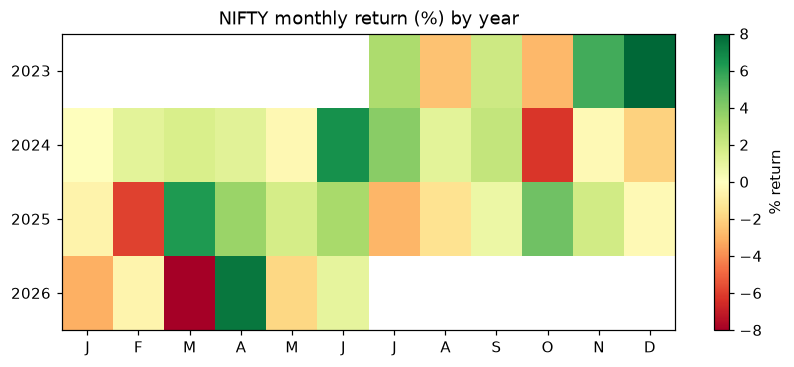
The chart is saved next to the script as a PNG, and the portal embeds it automatically. Scan down any column: if April is green most years, the seasonal story holds together; if it's a patchwork, be sceptical.
Try it yourself
- Swap
NIFTYforBANKNIFTYonNSE_INDEXin the weekday example. Does the strongest weekday change? - In the turn-of-month example, widen the window to the last three and first four days and see whether the effect grows or fades.
- Change the seasonal backtest to go long only in historically strong months instead of weekdays, and compare the equity curve.
Recap
- Seasonality measures whether the calendar itself tilts returns; it is real but small and noisy.
- Everything starts with daily returns via
pct_change(), then agroupbyon the date index does the heavy lifting. index.dayofweekandindex.monthunlock day-of-week and month-of-year effects in a couple of lines.cumcount()over a monthly period ranks days within a month - the key to the turn-of-month test.- Boolean masks combined with
&/|/~are the bridge from analysis to a tradable rule. - Discover calendar facts like the expiry weekday at runtime instead of hard-coding them.
- Compounding masked returns with
(1 + ret).cumprod()gives an equity curve - but beware fitting and testing on the same data.
Next we leave history behind and step into the options market itself - reading the chain, resolving real strikes, understanding the greeks, and placing multi-leg orders, all safely in analyze mode.