Charting with Matplotlib
Static charts: price lines, return distributions, subplots and indicator overlays.
- ·Line & step charts
- ·Subplots
- ·Return histograms
- ·Seaborn statistical charts
- ·Correlation heatmaps
- ·Save figures to file
A table of numbers is honest, but it's slow to read. Your eye can take in a chart in a second - a trend, a spike, a quiet stretch of consolidation - that would take a minute of squinting at rows. That's why every trader lives on charts, and why turning your Pandas DataFrames into pictures is one of the most useful skills in this whole series.
The tool for that is Matplotlib, the original and most widely used plotting library in Python. It's not the flashiest, but it's everywhere, it's dependable, and it draws exactly what you tell it to. In this chapter we'll build the charts you'll actually reach for: a clean price line, price stacked over volume, a histogram of returns, moving averages laid over price, buy and sell markers at crossover points, a hand-built candlestick chart, an equity curve, and a drawdown panel. Then we bring in Seaborn, a library built on top of Matplotlib that makes statistical charts (distributions, correlation heatmaps, box plots) look polished with almost no effort. We mix in an MCX commodity and an index so you see it all works beyond equities.
Drawing to a file, not a window
Here's the one habit that makes Matplotlib painless in this course. Normally Matplotlib tries to pop open a window to show your chart - which is useless on a server, in a script, or anywhere headless. So we tell it to draw to an image file instead. Every example in this chapter ends the same way:
out = Path(__file__).with_suffix(".png")
plt.savefig(out, dpi=110, bbox_inches="tight")
print("Saved", out.name)
Path(__file__).with_suffix(".png") just means "a PNG file with the same name as this script, sitting right next to it." dpi=110 controls sharpness; bbox_inches="tight" trims the whitespace. The portal then automatically embeds that PNG below each example, so the chart you generate is the chart you see on this page.
The example runner forces Matplotlib's non-interactive Agg backend (MPLBACKEND=Agg), which draws straight to a file with no window. That's why every script here just needs import matplotlib.pyplot as plt and a savefig at the end - no display, no blocking. If you run these on your own machine and a window helps, you can drop the backend setting, but saving to PNG always works.
A line of closing prices
The simplest useful chart is a line of the closing price over time. The pattern has three steps you'll repeat in every example: create a figure and an axes (the drawing area) with plt.subplots(), call ax.plot(x, y) to draw, then dress it up with a title, labels and a grid. Instead of feeding the raw dates as the x-axis, we plot against an evenly spaced position for each trading day and then label a few of those positions with their dates; the close column is the y-axis.
# Your first chart: a line of closing prices, saved as a PNG.
# We plot against an evenly-spaced position (0,1,2,...) and label ticks with dates,
# so non-trading days leave no gap.
import os
from datetime import datetime, timedelta
from pathlib import Path

import matplotlib.pyplot as plt
from openalgo import api

client = api(
    api_key=os.getenv("OPENALGO_API_KEY", "your_api_key_here"),
    host=os.getenv("OPENALGO_HOST", "http://127.0.0.1:5000"),
)

end = datetime.now().strftime("%Y-%m-%d")
start = (datetime.now() - timedelta(days=120)).strftime("%Y-%m-%d")
df = client.history(symbol="RELIANCE", exchange="NSE", interval="D", start_date=start, end_date=end)
x = list(range(len(df)))

fig, ax = plt.subplots(figsize=(9, 4))
ax.plot(x, df["close"], color="#1f6feb", linewidth=1.6)
ax.set_title("RELIANCE daily close")
ax.set_ylabel("Price")
ax.grid(True, alpha=0.3)

step = max(1, len(df) // 8)
ax.set_xticks(x[::step])
ax.set_xticklabels(df.index[::step].strftime("%d %b"), rotation=45, ha="right")

out = Path(__file__).with_suffix(".png")
plt.savefig(out, dpi=110, bbox_inches="tight")
print("Saved", out.name)Saved 01_line_close.png
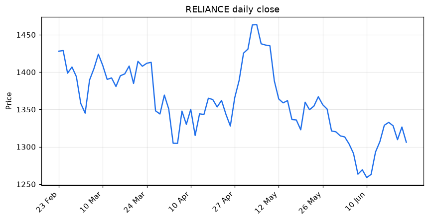
Why positions instead of dates? Markets are shut on weekends and holidays, so a true date axis leaves ugly blank gaps (very obvious on candlesticks and volume bars). By plotting against range(len(df)) and relabelling a handful of ticks with df.index[::step].strftime("%d %b"), every trading day sits flush against the next - no gaps - while you still read real dates along the bottom. We use this same trick on every time chart in the chapter.
fig, ax = plt.subplots() is the line you'll start almost every chart with. fig is the whole canvas; ax is the panel you draw on. Keeping a named ax makes everything afterward - titles, grids, extra lines - a tidy ax.something(...) call instead of a tangle of global commands.
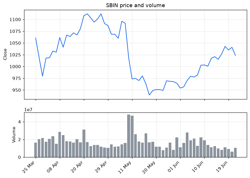
Price over volume: subplots
Price and volume belong together - a breakout on heavy volume means more than one on a quiet day. To show both without cramming them onto one scale, we use subplots: two stacked panels sharing the same x-axis. plt.subplots(2, 1, sharex=True) makes two rows; height_ratios=[2, 1] makes the price panel twice as tall as the volume panel. Price goes on top as a line, volume below as bars.
# Two stacked panels: price on top, volume bars below. A positional x keeps the
# volume bars evenly spaced with no weekend gaps.
import os
from datetime import datetime, timedelta
from pathlib import Path

import matplotlib.pyplot as plt
from openalgo import api

client = api(
    api_key=os.getenv("OPENALGO_API_KEY", "your_api_key_here"),
    host=os.getenv("OPENALGO_HOST", "http://127.0.0.1:5000"),
)

end = datetime.now().strftime("%Y-%m-%d")
start = (datetime.now() - timedelta(days=90)).strftime("%Y-%m-%d")
df = client.history(symbol="SBIN", exchange="NSE", interval="D", start_date=start, end_date=end)
x = list(range(len(df)))

fig, (ax1, ax2) = plt.subplots(2, 1, figsize=(9, 6), sharex=True,
                               gridspec_kw={"height_ratios": [2, 1]})
ax1.plot(x, df["close"], color="#1f6feb")
ax1.set_title("SBIN price and volume")
ax1.set_ylabel("Close")
ax1.grid(True, alpha=0.3)

ax2.bar(x, df["volume"], color="#8b949e")
ax2.set_ylabel("Volume")
ax2.grid(True, alpha=0.3)

step = max(1, len(df) // 8)
ax2.set_xticks(x[::step])
ax2.set_xticklabels(df.index[::step].strftime("%d %b"), rotation=45, ha="right")

out = Path(__file__).with_suffix(".png")
plt.savefig(out, dpi=110, bbox_inches="tight")
print("Saved", out.name)Saved 02_price_volume.png
A histogram of daily returns
A histogram answers a different question: not "what happened when?" but "how are the daily moves distributed?" It sorts every daily return into bins and draws a bar for how many days landed in each. The result is the shape of the stock's risk - a tall narrow peak means most days are calm; fat tails mean big moves are common. We mark the zero line (break-even) and the average so you can see any tilt.
# A histogram shows how daily returns are spread -- the shape of risk.
import os
from datetime import datetime, timedelta
from pathlib import Path

import matplotlib.pyplot as plt
from openalgo import api

client = api(
    api_key=os.getenv("OPENALGO_API_KEY", "your_api_key_here"),
    host=os.getenv("OPENALGO_HOST", "http://127.0.0.1:5000"),
)

end = datetime.now().strftime("%Y-%m-%d")
start = (datetime.now() - timedelta(days=250)).strftime("%Y-%m-%d")
df = client.history(symbol="INFY", exchange="NSE", interval="D", start_date=start, end_date=end)

rets = df["close"].pct_change().dropna() * 100   # daily returns in percent

fig, ax = plt.subplots(figsize=(8, 4.5))
ax.hist(rets, bins=30, color="#1f6feb", edgecolor="white")
ax.axvline(0, color="#8b949e", linestyle="--")          # the break-even line
ax.axvline(rets.mean(), color="#d29922", label=f"mean {rets.mean():.2f}%")
ax.set_title("INFY daily return distribution")
ax.set_xlabel("Daily return (%)")
ax.set_ylabel("Number of days")
ax.legend()

out = Path(__file__).with_suffix(".png")
plt.savefig(out, dpi=110, bbox_inches="tight")
print("Saved", out.name, "from", len(rets), "days")Saved 03_returns_histogram.png from 167 days
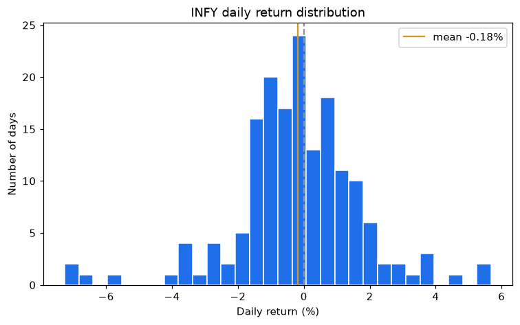
The width of that distribution is volatility, drawn out for your eye. A wide, spread-out histogram is a jumpy instrument; a tight one is calm. When we compute volatility numbers later, this picture is what they're summarising in a single figure.
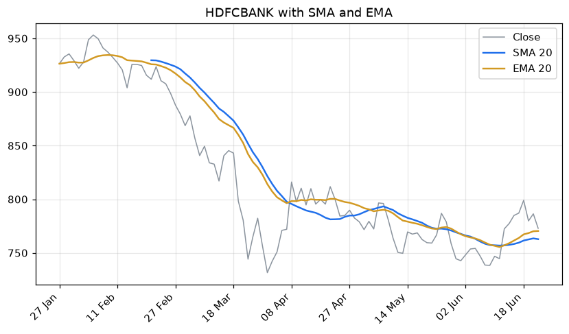
Overlaying moving averages
Now we layer information. Calling ax.plot() more than once on the same axes draws several lines together - so we plot the close faintly in grey, then lay a 20-day SMA and a 20-day EMA on top in bold colours. We pull both averages from the openalgo.ta indicator library you met earlier: ta.sma() weights every day equally, while ta.ema() (exponential) leans on recent prices and so turns faster. Seeing them on the same chart makes the difference obvious.
# Overlay a 20-day SMA and a 20-day EMA on price, using openalgo.ta.
import os
from datetime import datetime, timedelta
from pathlib import Path

import matplotlib.pyplot as plt
from openalgo import api, ta

client = api(
    api_key=os.getenv("OPENALGO_API_KEY", "your_api_key_here"),
    host=os.getenv("OPENALGO_HOST", "http://127.0.0.1:5000"),
)

end = datetime.now().strftime("%Y-%m-%d")
start = (datetime.now() - timedelta(days=150)).strftime("%Y-%m-%d")
df = client.history(symbol="HDFCBANK", exchange="NSE", interval="D", start_date=start, end_date=end)
x = list(range(len(df)))

df["sma20"] = ta.sma(df["close"], 20)   # simple average, equal weight
df["ema20"] = ta.ema(df["close"], 20)   # exponential, reacts faster to new prices

fig, ax = plt.subplots(figsize=(9, 4.5))
ax.plot(x, df["close"], color="#8b949e", linewidth=1, label="Close")
ax.plot(x, df["sma20"], color="#1f6feb", linewidth=1.6, label="SMA 20")
ax.plot(x, df["ema20"], color="#d29922", linewidth=1.6, label="EMA 20")
ax.set_title("HDFCBANK with SMA and EMA")
ax.legend()
ax.grid(True, alpha=0.3)

step = max(1, len(df) // 8)
ax.set_xticks(x[::step])
ax.set_xticklabels(df.index[::step].strftime("%d %b"), rotation=45, ha="right")

out = Path(__file__).with_suffix(".png")
plt.savefig(out, dpi=110, bbox_inches="tight")
print("Saved", out.name)Saved 04_overlay_sma_ema.png
Marking crossover signals
A chart earns its keep when it shows you where the rules fired. Here we compute a fast and a slow EMA, then use ta.crossover() and ta.crossunder() to find the exact days the fast line crosses the slow one - the heart of a moving-average system. ax.scatter() drops a green up-triangle on each buy day and a red down-triangle on each sell day, placed at that day's close. Suddenly an abstract signal becomes something you can eyeball against the price action.
# Mark where a fast average crosses a slow one: the signal on the chart.
import os
from datetime import datetime, timedelta
from pathlib import Path

import matplotlib.pyplot as plt
from openalgo import api, ta

client = api(
    api_key=os.getenv("OPENALGO_API_KEY", "your_api_key_here"),
    host=os.getenv("OPENALGO_HOST", "http://127.0.0.1:5000"),
)

end = datetime.now().strftime("%Y-%m-%d")
start = (datetime.now() - timedelta(days=250)).strftime("%Y-%m-%d")
df = client.history(symbol="ICICIBANK", exchange="NSE", interval="D", start_date=start, end_date=end)
x = list(range(len(df)))

df["fast"] = ta.ema(df["close"], 10)
df["slow"] = ta.ema(df["close"], 30)
df["buy"] = ta.crossover(df["fast"], df["slow"])
df["sell"] = ta.crossunder(df["fast"], df["slow"])
buy_pos = [i for i, b in enumerate(df["buy"]) if b]      # positions, not dates
sell_pos = [i for i, s in enumerate(df["sell"]) if s]

fig, ax = plt.subplots(figsize=(9, 4.5))
ax.plot(x, df["close"], color="#8b949e", linewidth=1, label="Close")
ax.plot(x, df["fast"], color="#1f6feb", linewidth=1.2, label="EMA 10")
ax.plot(x, df["slow"], color="#d29922", linewidth=1.2, label="EMA 30")
ax.scatter(buy_pos, df["close"].iloc[buy_pos], marker="^", color="#2ea043", s=90, label="Buy", zorder=5)
ax.scatter(sell_pos, df["close"].iloc[sell_pos], marker="v", color="#cf222e", s=90, label="Sell", zorder=5)
ax.set_title("ICICIBANK EMA crossover signals")
ax.legend()
ax.grid(True, alpha=0.3)

step = max(1, len(df) // 8)
ax.set_xticks(x[::step])
ax.set_xticklabels(df.index[::step].strftime("%d %b"), rotation=45, ha="right")

out = Path(__file__).with_suffix(".png")
plt.savefig(out, dpi=110, bbox_inches="tight")
print("Saved", out.name, "with", len(buy_pos), "buys and", len(sell_pos), "sells")Saved 05_mark_crossovers.png with 6 buys and 5 sells
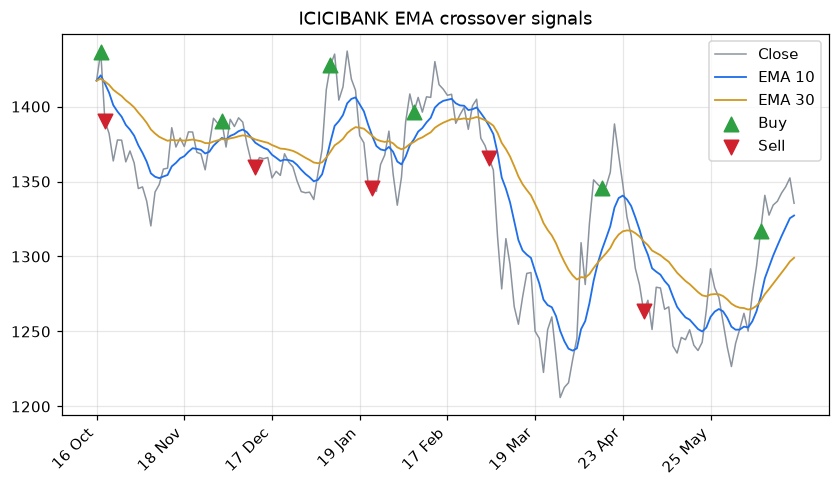
These markers sit on the day the signal formed, which uses that day's close - fine for visualising. In a real backtest you'd act on the next bar's open, because you can't trade on a close you haven't seen yet. We tackle that look-ahead trap properly in the signals and backtesting chapters; for now, just know the chart and the tradeable moment differ by a bar.
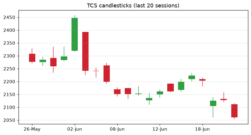
A candlestick chart by hand
Matplotlib has no built-in candlestick, which turns out to be a great lesson: a candle is just a thin line from low to high (the wick) plus a fat bar from open to close (the body), coloured green when the close beats the open and red when it doesn't. We loop over the last twenty sessions and draw each one. It's a few more lines than the rest, but it demystifies a chart you've stared at for years - and shows you can draw anything once you break it into rectangles and lines.
# A hand-built candlestick chart -- one rectangle and wick per session.
import os
from datetime import datetime, timedelta
from pathlib import Path

import matplotlib.pyplot as plt
from openalgo import api

client = api(
    api_key=os.getenv("OPENALGO_API_KEY", "your_api_key_here"),
    host=os.getenv("OPENALGO_HOST", "http://127.0.0.1:5000"),
)

end = datetime.now().strftime("%Y-%m-%d")
start = (datetime.now() - timedelta(days=40)).strftime("%Y-%m-%d")
df = client.history(symbol="TCS", exchange="NSE", interval="D", start_date=start, end_date=end).tail(20)

fig, ax = plt.subplots(figsize=(9, 4.5))
for i, (_, row) in enumerate(df.iterrows()):
    up = row["close"] >= row["open"]
    colour = "#2ea043" if up else "#cf222e"          # green up day, red down day
    ax.plot([i, i], [row["low"], row["high"]], color=colour, linewidth=1)        # the wick
    lo, hi = sorted([row["open"], row["close"]])
    ax.bar(i, hi - lo, bottom=lo, width=0.6, color=colour)                       # the body

ax.set_title("TCS candlesticks (last 20 sessions)")
ax.set_xticks(range(0, len(df), 4))
ax.set_xticklabels([d.strftime("%d-%b") for d in df.index[::4]])
ax.grid(True, axis="y", alpha=0.3)

out = Path(__file__).with_suffix(".png")
plt.savefig(out, dpi=110, bbox_inches="tight")
print("Saved", out.name)Saved 06_candlestick.png
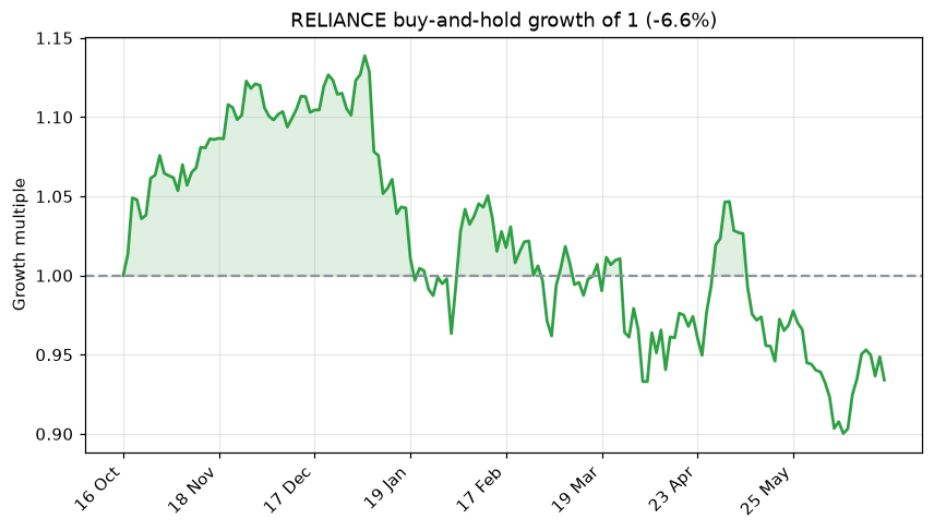
The equity curve
.cumprod() from the last chapter turned daily returns into a growth curve; now we draw it. This equity curve shows what one rupee of buy-and-hold would have become over the window, with a dashed line at 1.0 for break-even and the area above it shaded green. This exact picture - a line that hopefully climbs from left to right - is how you'll judge every strategy from the backtesting chapters onward.
# The equity curve: what buy-and-hold would have done to your capital.
import os
from datetime import datetime, timedelta
from pathlib import Path

import matplotlib.pyplot as plt
from openalgo import api

client = api(
    api_key=os.getenv("OPENALGO_API_KEY", "your_api_key_here"),
    host=os.getenv("OPENALGO_HOST", "http://127.0.0.1:5000"),
)

end = datetime.now().strftime("%Y-%m-%d")
start = (datetime.now() - timedelta(days=250)).strftime("%Y-%m-%d")
df = client.history(symbol="RELIANCE", exchange="NSE", interval="D", start_date=start, end_date=end)
x = list(range(len(df)))

rets = df["close"].pct_change().fillna(0)
growth = (1 + rets).cumprod().values          # 1.0 at the start; compounds each day

fig, ax = plt.subplots(figsize=(9, 4.5))
ax.plot(x, growth, color="#2ea043", linewidth=1.8)
ax.axhline(1.0, color="#8b949e", linestyle="--")     # break-even line
ax.fill_between(x, 1.0, growth, where=growth >= 1.0, color="#2ea043", alpha=0.15)
ax.set_title(f"RELIANCE buy-and-hold growth of 1 ({(growth[-1]-1)*100:.1f}%)")
ax.set_ylabel("Growth multiple")
ax.grid(True, alpha=0.3)

step = max(1, len(df) // 8)
ax.set_xticks(x[::step])
ax.set_xticklabels(df.index[::step].strftime("%d %b"), rotation=45, ha="right")

out = Path(__file__).with_suffix(".png")
plt.savefig(out, dpi=110, bbox_inches="tight")
print("Saved", out.name)Saved 07_cumulative_returns.png
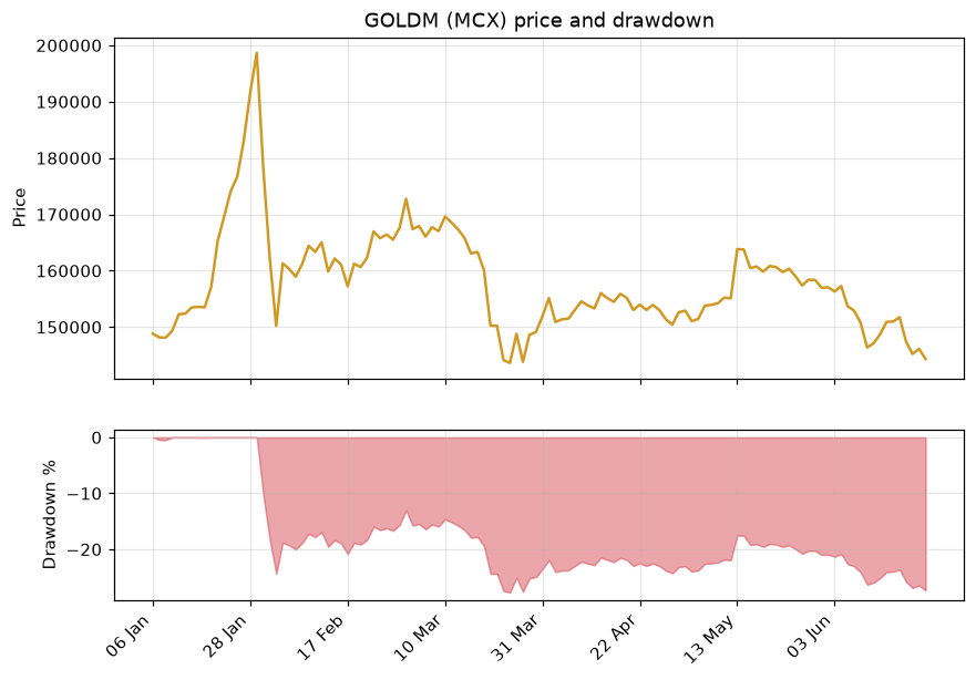
An MCX commodity: price with drawdown
To prove none of this is equity-only, we chart GOLDM, a gold contract on the MCX commodity exchange, in two panels. The top shows price; the bottom shades the drawdown - how far below its running peak the contract sits on each day, computed with .cummax() as in Chapter 7. A drawdown panel under the price is one of the most informative views in trading: it makes the pain of every dip impossible to ignore.
# An MCX commodity chart: GOLDM price with its drawdown shaded beneath.
import os
from datetime import datetime, timedelta
from pathlib import Path

import matplotlib.pyplot as plt
from openalgo import api

client = api(
    api_key=os.getenv("OPENALGO_API_KEY", "your_api_key_here"),
    host=os.getenv("OPENALGO_HOST", "http://127.0.0.1:5000"),
)

end = datetime.now().strftime("%Y-%m-%d")
start = (datetime.now() - timedelta(days=180)).strftime("%Y-%m-%d")
df = client.history(symbol="GOLDM03JUL26FUT", exchange="MCX", interval="D", start_date=start, end_date=end)
x = list(range(len(df)))

df["dd"] = (df["close"] / df["close"].cummax() - 1) * 100   # % below the running peak

fig, (ax1, ax2) = plt.subplots(2, 1, figsize=(9, 6), sharex=True,
                               gridspec_kw={"height_ratios": [2, 1]})
ax1.plot(x, df["close"], color="#d29922", linewidth=1.6)
ax1.set_title("GOLDM (MCX) price and drawdown")
ax1.set_ylabel("Price")
ax1.grid(True, alpha=0.3)

ax2.fill_between(x, df["dd"], 0, color="#cf222e", alpha=0.4)
ax2.set_ylabel("Drawdown %")
ax2.grid(True, alpha=0.3)

step = max(1, len(df) // 8)
ax2.set_xticks(x[::step])
ax2.set_xticklabels(df.index[::step].strftime("%d %b"), rotation=45, ha="right")

out = Path(__file__).with_suffix(".png")
plt.savefig(out, dpi=110, bbox_inches="tight")
print("Saved", out.name, "| deepest drawdown", round(df["dd"].min(), 2), "%")Saved 08_mcx_gold_drawdown.png | deepest drawdown -27.7 %
Comparing two symbols fairly
You can't fairly compare a 2000-rupee stock with a 1000-rupee one by plotting their raw prices - the expensive one just looks bigger. The fix is rebasing: divide each price series by its own first value and multiply by 100, so both start at exactly 100 and the chart shows pure relative performance. Whichever line ends higher was the better hold over the window, regardless of nominal price.
# Compare two stocks fairly by rebasing both to 100 on day one.
import os
from datetime import datetime, timedelta
from pathlib import Path

import matplotlib.pyplot as plt
from openalgo import api

client = api(
    api_key=os.getenv("OPENALGO_API_KEY", "your_api_key_here"),
    host=os.getenv("OPENALGO_HOST", "http://127.0.0.1:5000"),
)

end = datetime.now().strftime("%Y-%m-%d")
start = (datetime.now() - timedelta(days=180)).strftime("%Y-%m-%d")


def rebased(sym):
    d = client.history(symbol=sym, exchange="NSE", interval="D", start_date=start, end_date=end)
    return d["close"] / d["close"].iloc[0] * 100      # everyone starts at 100

series = {sym: rebased(sym) for sym in ["TCS", "INFY"]}
idx = next(iter(series.values())).index
x = list(range(len(idx)))

fig, ax = plt.subplots(figsize=(9, 4.5))
for (sym, s), colour in zip(series.items(), ["#1f6feb", "#d29922"]):
    ax.plot(x, s.values, label=sym, color=colour, linewidth=1.6)

ax.axhline(100, color="#8b949e", linestyle="--")
ax.set_title("TCS vs INFY relative performance (rebased to 100)")
ax.set_ylabel("Index (start = 100)")
ax.legend()
ax.grid(True, alpha=0.3)

step = max(1, len(idx) // 8)
ax.set_xticks(x[::step])
ax.set_xticklabels(idx[::step].strftime("%d %b"), rotation=45, ha="right")

out = Path(__file__).with_suffix(".png")
plt.savefig(out, dpi=110, bbox_inches="tight")
print("Saved", out.name)Saved 09_compare_normalized.png
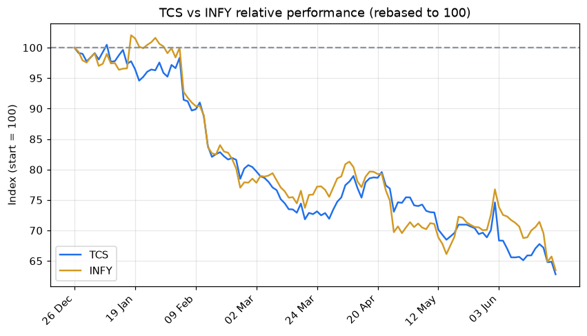
Rebasing to a common start (often 100) is how every "stock vs index" or "fund vs benchmark" chart you've seen is built. It strips away the price level and leaves only the thing you care about: who grew more, and how smoothly.
Seeing patterns with Seaborn
Matplotlib draws anything, but you do the styling. Seaborn sits on top of it and ships beautiful defaults plus ready-made statistical charts, so one line gets you a polished result. It's perfect for the questions traders actually ask: how are my returns spread, which stocks move together, and are there calendar patterns? Install it once with uv add seaborn, then import seaborn as sns.
First, the return distribution again, but richer: sns.histplot(..., kde=True) overlays a smooth KDE (kernel density estimate) curve, a clean outline of the shape of risk. Here on a volatile MCX crude oil contract.
# Seaborn makes statistical charts beautiful by default. Here: a return distribution
# with a smooth density curve (KDE) laid over the histogram.
import os
from datetime import datetime, timedelta
from pathlib import Path

import matplotlib.pyplot as plt
import seaborn as sns
from openalgo import api

client = api(
    api_key=os.getenv("OPENALGO_API_KEY", "your_api_key_here"),
    host=os.getenv("OPENALGO_HOST", "http://127.0.0.1:5000"),
)

end = datetime.now().strftime("%Y-%m-%d")
start = (datetime.now() - timedelta(days=180)).strftime("%Y-%m-%d")
df = client.history(symbol="CRUDEOIL20JUL26FUT", exchange="MCX", interval="D", start_date=start, end_date=end)
rets = df["close"].pct_change().dropna() * 100   # daily returns in percent

sns.set_theme(style="darkgrid")
fig, ax = plt.subplots(figsize=(8, 4.5))
sns.histplot(rets, bins=30, kde=True, color="#d29922", ax=ax)
ax.axvline(0, color="grey", linestyle="--")
ax.set_title("CRUDEOIL daily return distribution (Seaborn)")
ax.set_xlabel("Daily return (%)")

out = Path(__file__).with_suffix(".png")
plt.savefig(out, dpi=110, bbox_inches="tight")
print("Saved", out.name, "| std dev", round(rets.std(), 2), "%")Saved 10_seaborn_returns_kde.png | std dev 3.43 %
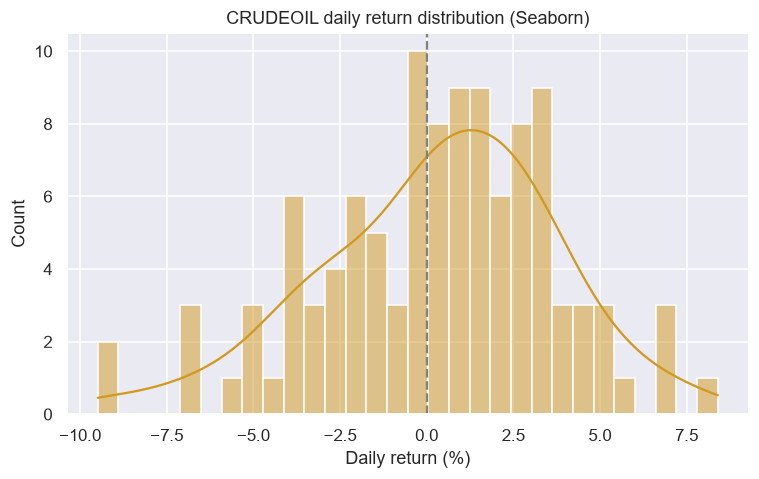
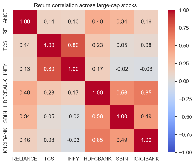
A correlation heatmap is one of the most useful pictures in portfolio work. sns.heatmap() colours a grid of correlations: stocks that move together glow warm (near +1), genuinely diversifying pairs stay cool. If everything in your basket is dark red, you are less diversified than you think.
# A correlation heatmap shows which stocks move together. Diversification lives
# in the cool-coloured (low correlation) pairs.
import os
from datetime import datetime, timedelta
from pathlib import Path

import matplotlib.pyplot as plt
import pandas as pd
import seaborn as sns
from openalgo import api

client = api(
    api_key=os.getenv("OPENALGO_API_KEY", "your_api_key_here"),
    host=os.getenv("OPENALGO_HOST", "http://127.0.0.1:5000"),
)

end = datetime.now().strftime("%Y-%m-%d")
start = (datetime.now() - timedelta(days=180)).strftime("%Y-%m-%d")
syms = ["RELIANCE", "TCS", "INFY", "HDFCBANK", "SBIN", "ICICIBANK"]
closes = {s: client.history(symbol=s, exchange="NSE", interval="D",
                            start_date=start, end_date=end)["close"] for s in syms}
rets = pd.DataFrame(closes).pct_change().dropna()

sns.set_theme(style="white")
fig, ax = plt.subplots(figsize=(7, 5.5))
sns.heatmap(rets.corr(), annot=True, fmt=".2f", cmap="coolwarm", vmin=-1, vmax=1, ax=ax)
ax.set_title("Return correlation across large-cap stocks")

out = Path(__file__).with_suffix(".png")
plt.savefig(out, dpi=110, bbox_inches="tight")
print("Saved", out.name)Saved 11_seaborn_corr_heatmap.png
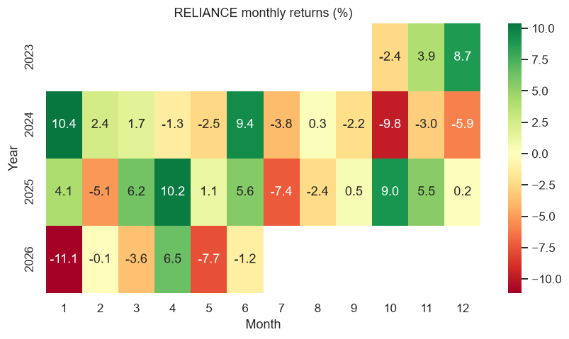
The same heatmap idea, applied to the calendar, reveals seasonality: each cell is one month's return, green for gains and red for losses, with years down the side and months across the top. Patches of colour hint at recurring strong or weak months (we dig into this properly in the seasonal-strategies chapter).
# A month-by-year heatmap of returns: spot seasonal strength and weak patches at a glance.
import os
from datetime import datetime, timedelta
from pathlib import Path

import matplotlib.pyplot as plt
import seaborn as sns
from openalgo import api

client = api(
    api_key=os.getenv("OPENALGO_API_KEY", "your_api_key_here"),
    host=os.getenv("OPENALGO_HOST", "http://127.0.0.1:5000"),
)

end = datetime.now().strftime("%Y-%m-%d")
start = (datetime.now() - timedelta(days=1000)).strftime("%Y-%m-%d")
df = client.history(symbol="RELIANCE", exchange="NSE", interval="D", start_date=start, end_date=end)

monthly = df["close"].resample("ME").last().pct_change().dropna() * 100
table = monthly.groupby([monthly.index.year, monthly.index.month]).first().unstack(level=1)
table.index.name, table.columns.name = "Year", "Month"

sns.set_theme(style="white")
fig, ax = plt.subplots(figsize=(9, 4.5))
sns.heatmap(table, annot=True, fmt=".1f", cmap="RdYlGn", center=0, ax=ax)
ax.set_title("RELIANCE monthly returns (%)")

out = Path(__file__).with_suffix(".png")
plt.savefig(out, dpi=110, bbox_inches="tight")
print("Saved", out.name)Saved 12_seaborn_monthly_heatmap.png
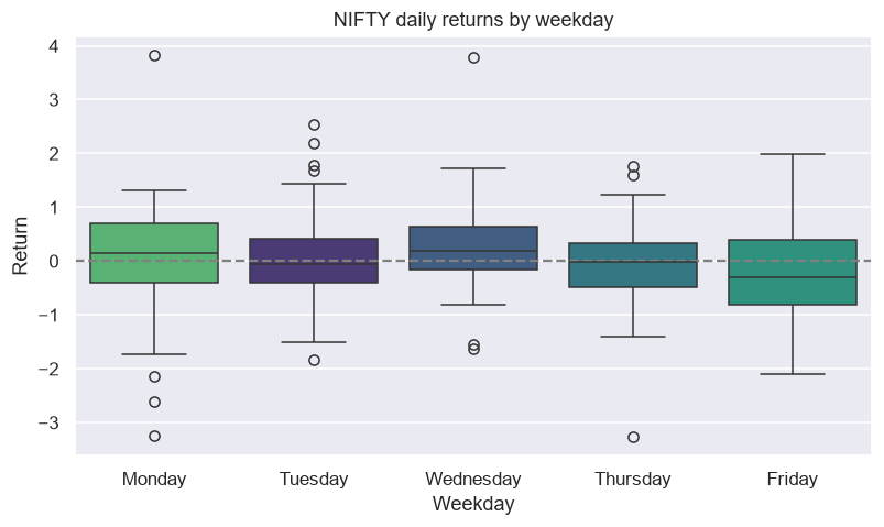
Finally a box plot, which summarises a whole distribution in one shape: the box is the middle half of the data, the line inside is the median, and dots are outliers. Splitting NIFTY's daily returns by weekday lets you eyeball whether any day really behaves differently.
# A box plot of returns by weekday: does any day behave differently? Seaborn shows
# the spread, the median, and the outliers all at once.
import os
from datetime import datetime, timedelta
from pathlib import Path

import matplotlib.pyplot as plt
import pandas as pd
import seaborn as sns
from openalgo import api

client = api(
    api_key=os.getenv("OPENALGO_API_KEY", "your_api_key_here"),
    host=os.getenv("OPENALGO_HOST", "http://127.0.0.1:5000"),
)

end = datetime.now().strftime("%Y-%m-%d")
start = (datetime.now() - timedelta(days=500)).strftime("%Y-%m-%d")
df = client.history(symbol="NIFTY", exchange="NSE_INDEX", interval="D", start_date=start, end_date=end)
rets = df["close"].pct_change().dropna() * 100

data = pd.DataFrame({"Weekday": rets.index.day_name(), "Return": rets.values})
order = ["Monday", "Tuesday", "Wednesday", "Thursday", "Friday"]

sns.set_theme(style="darkgrid")
fig, ax = plt.subplots(figsize=(8.5, 4.5))
sns.boxplot(data=data, x="Weekday", y="Return", order=order, hue="Weekday", palette="viridis", legend=False, ax=ax)
ax.axhline(0, color="grey", linestyle="--")
ax.set_title("NIFTY daily returns by weekday")

out = Path(__file__).with_suffix(".png")
plt.savefig(out, dpi=110, bbox_inches="tight")
print("Saved", out.name)Saved 13_seaborn_weekday_box.png
Reach for Seaborn when the question is statistical (distributions, correlations, comparisons across groups) and for Matplotlib when you need precise control over a price chart. They share the same figure, so you can freely mix them.
Try it yourself
- Change the colour and
linewidthin the line-chart example, then add a second symbol's close on the same axes with anotherax.plot(). - In the candlestick example, change
.tail(20)to.tail(40)and adjust the barwidthso the candles don't overlap. - Take the crossover example and widen the averages to EMA 20 and EMA 50 - do you get fewer, cleaner signals?
Recap
- Force a file backend (the runner sets Agg) and end every script with
plt.savefig(Path(__file__).with_suffix(".png"), ...); the portal embeds the PNG. fig, ax = plt.subplots()is the universal starting point;ax.plot,ax.bar,ax.histandax.scatterare your core drawing tools.- Stack panels with
subplots(2, 1, sharex=True)andheight_ratiosfor price-over-volume or price-over-drawdown layouts. - Calling
ax.plot()repeatedly overlays lines - perfect for laying moving averages fromopenalgo.taover price. ax.scatter()marks signal points; a candlestick is just wicks (lines) plus bodies (bars), coloured by direction.- Cumulative returns draw an equity curve,
.cummax()draws drawdown, and rebasing to 100 compares symbols fairly. - Plot against evenly spaced positions (with date-labelled ticks) so non-trading days leave no gaps.
- Seaborn adds polished statistical charts in one line: KDE distributions, correlation and seasonality heatmaps, and box plots by group.
You now have the static-charting toolkit. Next we make charts you can zoom, pan and hover over: Chapter 9 builds interactive candlestick charts with Plotly.