The DataFrame

A single labelled column - a Series - is useful, but market data is a table: for every date there's an open, a high, a low, a close, and a volume, all in a row. Stack Series side by side, sharing one index, and you get the DataFrame - the single most important object in all of data analysis. If pandas is the engine of quant work, the DataFrame is the chassis. Spend real time here; almost everything that follows is just doing things to a DataFrame.

A DataFrame is a table

The wonderful thing is you've already been handed DataFrames - every yfinance history call returns one. Rows are dates (the index); columns are the OHLCV fields:

import yfinance as yf

# yfinance returns a DataFrame: rows are dates, columns are Open/High/Low/Close/Volume.
df = yf.Ticker("AAPL").history(period="6mo")
df = df[["Open", "High", "Low", "Close", "Volume"]].round(2)
df.index = df.index.date           # tidy the date index for display

print("Shape   :", df.shape)        # (rows, columns)
print("Columns :", list(df.columns))
print()
print("First 3 rows:")
print(df.head(3))

Shape   : (123, 5)
Columns : ['Open', 'High', 'Low', 'Close', 'Volume']

First 3 rows:
              Open    High     Low   Close    Volume
2025-12-26  273.65  274.86  272.35  272.89  21521800
2025-12-29  272.18  273.85  271.84  273.25  23715200
2025-12-30  272.30  273.57  271.78  272.57  22139600

df.shape told us (123, 5) - 123 days, 5 columns. df.columns lists the column names, and df.head(3) shows the first three rows. A DataFrame is, quite literally, a spreadsheet you drive with code.

Columns, rows, selecting and filtering

Three moves cover most of what you'll ever do to a DataFrame: pick columns, add columns, and filter rows:

import yfinance as yf

df = yf.Ticker("AAPL").history(period="3mo")[["Open", "Close", "Volume"]].round(2)
df.index = df.index.date

# One column is a Series; pick it with df["Close"].
print("Close column (last 3):")
print(df["Close"].tail(3))
print()

# Add a NEW column, computed from existing ones (open-to-close change).
df["Chg%"] = ((df["Close"] - df["Open"]) / df["Open"] * 100).round(2)

# Filter rows: keep only days that gained more than 2% from open to close.
big_up = df[df["Chg%"] > 2]
print("Days up more than 2% (open to close):")
print(big_up[["Close", "Chg%"]])

Close column (last 3):
2026-06-22    297.01
2026-06-23    294.30
2026-06-24    293.08
Name: Close, dtype: float64

Days up more than 2% (open to close):
             Close  Chg%
2026-03-31  253.56  2.37
2026-04-15  266.18  3.20
2026-05-05  283.92  2.62
2026-06-02  315.20  2.52

• Select one column with df["Close"] (you get a Series) or several with df[["Open", "Close"]] (a smaller DataFrame).
• Add a column just by assigning to a new name: df["Chg%"] = ..., computed from other columns - all vectorised, no loop.
• Filter rows with a condition in brackets: df[df["Chg%"] > 2] keeps only the days that gained more than 2%.

Quick inspection: look before you leap

Before analysing any dataset, eyeball it. A handful of methods tell you what you're dealing with:

• df.head() / df.tail() - first / last rows.
• df.shape - how many rows and columns.
• df.columns - the column names.
• df.info() - column types and how many values are missing.
• df.describe() - count, mean, min, max and quartiles for every numeric column at once.

This thirty-second habit catches missing data, wrong types and surprises before they corrupt your analysis - which is exactly the subject of Chapter 29.

A whole table, one chart

Because columns share an index, you can chart several together. Here the same DataFrame gives a price panel and a volume panel in one figure:

Copy

from pathlib import Path

import matplotlib

matplotlib.use("Agg")
import matplotlib.pyplot as plt
import seaborn as sns
import yfinance as yf

df = yf.Ticker("AAPL").history(period="6mo")

# Two columns of the same DataFrame, drawn as two stacked panels.
sns.set_theme(style="whitegrid")
fig, (ax1, ax2) = plt.subplots(
    2, 1, figsize=(8, 5), sharex=True, gridspec_kw={"height_ratios": [3, 1]}
)
ax1.plot(df.index, df["Close"], color="#7c83ff", lw=1.6)
ax1.set_title("AAPL - price and volume, last 6 months")
ax1.set_ylabel("Close (USD)")
ax2.bar(df.index, df["Volume"] / 1e6, color="#9aa0c4", width=1.0)
ax2.set_ylabel("Volume (M)")

out = Path(__file__).with_suffix(".png")
plt.savefig(out, dpi=110, bbox_inches="tight")
print("Rows plotted :", len(df))
print("Columns used :", ["Close", "Volume"])

Live output

Rows plotted : 123
Columns used : ['Close', 'Volume']

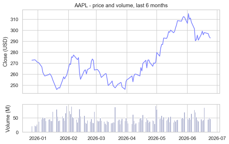
Two columns - Close and Volume - drawn from a single table, perfectly aligned on the same dates. That alignment, handled automatically by the shared index, is the quiet magic that makes the DataFrame so powerful.

More ways to slice a DataFrame

Selecting and filtering go a lot further than df["col"]. Four more tools cover almost everything you'll do day to day:

import numpy as np
import pandas as pd

df = pd.read_csv("reliance_6mo.csv", index_col="Date", parse_dates=True)

# .iloc selects by POSITION; .loc selects by LABEL.
print("First close (iloc[0])      :", df.iloc[0]["Close"])
print("Close on a date (loc)      :", df.loc["2026-06-24", "Close"])
print()

# Add a computed column, and a conditional one with np.where.
df["Range"] = df["High"] - df["Low"]
df["Day"] = np.where(df["Close"] >= df["Open"], "up", "down")

# sort_values ranks the whole table; here, the widest-range days.
print("Top 3 widest-range days:")
print(df.sort_values("Range", ascending=False).head(3)[["Close", "Range", "Day"]].round(2))
print()

# Filter on MULTIPLE conditions: & = and, | = or, each wrapped in ( ).
strong = df[(df["Day"] == "up") & (df["Range"] > 40)]
print("Up days with range > 40    :", len(strong))
print("Highest close              :", df["Close"].max(), "on", df["Close"].idxmax().date())

First close (iloc[0])      : 1551.03
Close on a date (loc)      : 1313.6

Top 3 widest-range days:
              Close  Range   Day
Date                            
2026-01-06  1500.66  72.37  down
2026-04-06  1298.70  68.69  down
2026-04-27  1359.51  60.32    up

Up days with range > 40    : 8
Highest close              : 1584.97 on 2026-01-02

• .iloc[] vs .loc[] - iloc selects by position (df.iloc[0], the first row), loc by label (df.loc["2026-06-24"], a specific date). This is the single most important distinction in pandas indexing.
• np.where(condition, a, b) builds a conditional column in one line - here tagging each day "up" or "down".
• .sort_values("col") ranks the whole table by a column (add ascending=False for biggest-first).
• Multiple-condition filters: combine masks with & (and) and | (or), wrapping each condition in brackets - df[(df["Day"] == "up") & (df["Range"] > 40)].

Slicing ranges of rows and columns

Beyond picking single rows, you can take ranges - and you give two slices at once, [rows, columns], just like a 2D NumPy array. .iloc slices by position (end excluded); .loc slices by label (end included):

import pandas as pd

df = pd.read_csv("reliance_6mo.csv", index_col="Date", parse_dates=True)

# .iloc = by POSITION (end excluded). Two slices: [rows, columns].
print("first 2 rows, by position:")
print(df.iloc[0:2, 0:4])          # rows 0-1, columns 0-3 (Open..Close)
print()

# .loc = by LABEL (end included). Slice a date range AND a column range.
print("a date range, columns Open..Close, by label:")
print(df.loc["2026-06-22":"2026-06-24", "Open":"Close"])

first 2 rows, by position:
               Open     High      Low    Close
Date                                          
2025-12-24  1565.46  1568.45  1546.45  1551.03
2025-12-26  1547.54  1553.82  1547.15  1552.02

a date range, columns Open..Close, by label:
              Open    High     Low   Close
Date                                      
2026-06-22  1316.7  1344.9  1314.1  1326.5
2026-06-23  1328.9  1333.0  1304.0  1309.5
2026-06-24  1305.7  1322.0  1297.5  1313.6

So df.iloc[0:2, 0:4] is "the first two rows and first four columns," and df.loc["2026-06-22":"2026-06-24", "Open":"Close"] is "those three dates, columns Open through Close." Same comma-separated [rows, columns] idea as NumPy - now with dates and column names as the labels.

Single vs MultiIndex columns (a yfinance gotcha)

Usually a DataFrame's columns are a simple flat list (Open, High, Close...). But sometimes columns have two levels - a MultiIndex - and this trips up everyone the first time, because yfinance returns one:

import yfinance as yf

# Ticker().history() gives SINGLE-level columns: Open, High, Low, Close, ...
hist = yf.Ticker("AAPL").history(period="5d")
print("history() columns :", list(hist.columns)[:5])
print("  hist['Close'] is a", type(hist["Close"]).__name__)
print()

# yf.download() gives a MULTI-INDEX: each column is a (field, ticker) pair.
dl = yf.download(["AAPL", "MSFT"], period="5d", progress=False)
print("download() columns:", list(dl.columns)[:4])
print("  dl['Close'] is a", type(dl["Close"]).__name__, "-> columns", list(dl["Close"].columns))
print("  one stock: dl['Close']['AAPL'].iloc[-1] =", round(float(dl["Close"]["AAPL"].dropna().iloc[-1]), 2))

history() columns : ['Open', 'High', 'Low', 'Close', 'Volume']
  hist['Close'] is a Series

download() columns: [('Close', 'AAPL'), ('Close', 'MSFT'), ('High', 'AAPL'), ('High', 'MSFT')]
  dl['Close'] is a DataFrame -> columns ['AAPL', 'MSFT']
  one stock: dl['Close']['AAPL'].iloc[-1] = 293.08

Here's the whole story: yf.Ticker("AAPL").history() gives plain columns, so df["Close"] is a Series (as you'd expect). But yf.download(...) gives a MultiIndex where each column is a (field, ticker) pair - so df["Close"] returns a whole DataFrame (one column per ticker), and you reach a single stock with a second key: df["Close"]["AAPL"].

Combining tables: concat and merge

Real analysis often means stitching tables together, and there are two distinct jobs. concat stacks tables (more rows); merge joins them on a shared key (more columns), exactly like a database JOIN:

import pandas as pd

# Two small tables about the same stocks.
prices = pd.DataFrame({"Symbol": ["RELIANCE", "TCS", "INFY"],
                       "Close": [1313.6, 2109.0, 1056.6]})
sectors = pd.DataFrame({"Symbol": ["RELIANCE", "TCS", "WIPRO"],
                        "Sector": ["Energy", "IT", "IT"]})

# concat: stack tables on top of each other (they share the same columns).
more = pd.DataFrame({"Symbol": ["HDFCBANK"], "Close": [1642.4]})
print("concat - stack the rows:")
print(pd.concat([prices, more], ignore_index=True))
print()

# merge: join two tables on a shared key column, like a database JOIN.
joined = prices.merge(sectors, on="Symbol", how="inner")   # inner = keep only matches
print("merge on Symbol (inner):")
print(joined)

concat - stack the rows:
     Symbol   Close
0  RELIANCE  1313.6
1       TCS  2109.0
2      INFY  1056.6
3  HDFCBANK  1642.4

merge on Symbol (inner):
     Symbol   Close  Sector
0  RELIANCE  1313.6  Energy
1       TCS  2109.0      IT

• pd.concat([a, b]) stacks rows - use it to glue together tables with the same columns (this quarter's data under last quarter's).
• a.merge(b, on="Symbol") lines up rows by a matching key column - here attaching each stock's sector to its price. The how argument controls what to keep: "inner" (only matches, as here), "left" (all of a), "outer" (everything). It's the spreadsheet VLOOKUP, done properly.

A DataFrame cheat-sheet

The greatest hits, grouped by job - know they exist, look up the details:

• Inspect: .head(), .tail(), .shape, .info(), .describe(), .columns, .dtypes
• Select & slice: df["col"], df[["a","b"]], .loc[rows, cols] (by label), .iloc[rows, cols] (by position), .at[] (one cell)
• Filter: df[mask], multi-condition with &/|, .query("col > 5"), .between()
• Add / change: df["new"] = ..., .assign(), np.where(), .rename(columns=...), .drop(columns=...)
• Order & rank: .sort_values(), .sort_index(), .nlargest(n, "col"), .nsmallest()
• Combine: pd.concat([a, b]) (stack rows), a.merge(b, on="key", how=...) (join on a key), a.join(b) (join on the index)
• Columns: flat vs MultiIndex (yf.download gives two-level (field, ticker)); flatten with df.xs(...) or df.droplevel(1, axis=1)
• Summarise: .sum(), .mean(), .groupby() (Chapter 31), .value_counts(), .corr() (column correlations)
• Apply your own logic: .apply(func) down columns, df["col"].map(...) per value

This is the working vocabulary of data analysis. You won't use all of it every day, but knowing the shape of what's available is exactly what lets you look up the rest.

Try it yourself

• Load 1 year of any stock with yf.Ticker("MSFT").history(period="1y") and print its .shape and .describe().
• Add a column df["Spread"] = df["High"] - df["Low"] (the daily range), then find the day with the largest spread.
• Filter for high-volume days: df[df["Volume"] > df["Volume"].mean()]. How many days traded above the average?

Recap

• A DataFrame is a table of named columns (each a Series) sharing one index - exactly what yfinance returns.
• Select columns with df["col"] / df[["a","b"]]; add a column by assigning to a new name; filter rows with boolean masks df[df["col"] > x].
• Inspect first with head, shape, columns, info, describe - it catches problems early.
• Columns share an index, so they align automatically - making multi-column maths and charts effortless.

You now know what a DataFrame is. The next practical questions are: how do you get one from anywhere - a CSV file, a download - and how do you save it? Chapter 28 is all about loading and storing market data, the gateway to working with your own datasets.