Loading Market Data

You know what a DataFrame is and what to do with one. The obvious next question: where do they come from? In practice, two places - a live download (we've been using yfinance) and a file on disk, almost always a CSV. Loading data is the very first line of every analysis, so this short, practical chapter makes sure you can always get a table in - and save one back out - whatever the source.

Fetching with yfinance, and saving a CSV

You've already fetched data with yfinance; here we add the other half - writing it to a CSV so you never have to download it again. We'll use an Indian stock this time:

import yfinance as yf

# ".NS" is Yahoo Finance's suffix for NSE-listed Indian stocks.
df = yf.Ticker("RELIANCE.NS").history(period="6mo")[["Open", "High", "Low", "Close", "Volume"]]
df = df.round(2).dropna()          # drop incomplete rows (Yahoo leaves today's bar empty)
df.index = df.index.date
df.index.name = "Date"

# Save the whole table to a CSV file - just one line.
df.to_csv("reliance_6mo.csv")
print("Saved", len(df), "rows to reliance_6mo.csv")
print(df.tail(3))

Saved 124 rows to reliance_6mo.csv
              Open    High     Low   Close    Volume
Date                                                
2026-06-22  1316.7  1344.9  1314.1  1326.5  12931213
2026-06-23  1328.9  1333.0  1304.0  1309.5  15400184
2026-06-24  1305.7  1322.0  1297.5  1313.6  11030917

Two India-specific notes. First, Yahoo's code for an NSE stock is the symbol plus .NS (so RELIANCE.NS) - we'll map symbols across sources properly in Chapter 34. Second, .dropna(): Yahoo often leaves the current day's bar empty until the close, so we drop incomplete rows - a small but important habit with Indian data, and the heart of the next chapter. Then df.to_csv("reliance_6mo.csv") writes the whole table to disk in one line.

Reading a CSV back

To load that file - or any CSV someone hands you - use pd.read_csv. Two arguments earn their keep with time-series data:

import pandas as pd

# Read the CSV back into a DataFrame, using the Date column as the index.
df = pd.read_csv("reliance_6mo.csv", index_col="Date", parse_dates=True)

print("Shape   :", df.shape)
print("Columns :", list(df.columns))
print()
print("Most recent rows:")
print(df.tail(3))
print()
print("Close-price summary:")
print(df["Close"].describe().round(2))

Shape   : (124, 5)
Columns : ['Open', 'High', 'Low', 'Close', 'Volume']

Most recent rows:
              Open    High     Low   Close    Volume
Date                                                
2026-06-22  1316.7  1344.9  1314.1  1326.5  12931213
2026-06-23  1328.9  1333.0  1304.0  1309.5  15400184
2026-06-24  1305.7  1322.0  1297.5  1313.6  11030917

Close-price summary:
count     124.00
mean     1388.35
std        69.07
min      1258.80
25%      1338.58
50%      1384.30
75%      1428.84
max      1584.97
Name: Close, dtype: float64

index_col="Date" tells pandas to use the Date column as the row index (instead of a plain 0,1,2 counter), and parse_dates=True turns those date strings into real datetime objects you can do time maths on. With those two, your loaded table behaves exactly like a freshly downloaded one.

describe(): the thirty-second X-ray

Notice the last line of that example: df["Close"].describe(). It returns a whole statistical summary at once - count, mean, standard deviation, min, max, and the quartiles. For our Reliance data it instantly reveals the six-month range (a low near 1259, a high near 1585) and the typical level (~1388). Run describe() on any new dataset before anything else; it's the fastest way to understand what you're holding and to spot anything odd.

From file to chart

Once a CSV is saved, you never need the internet again - load and chart entirely offline:

Copy

from pathlib import Path

import matplotlib

matplotlib.use("Agg")
import matplotlib.pyplot as plt
import pandas as pd
import seaborn as sns

# Load straight from the CSV - no internet needed once it is saved.
df = pd.read_csv("reliance_6mo.csv", index_col="Date", parse_dates=True)

sns.set_theme(style="whitegrid")
fig, ax = plt.subplots(figsize=(8, 4))
ax.plot(df.index, df["Close"], color="#21c87a", lw=1.7)
ax.set_title("RELIANCE (NSE) - close, last 6 months")
ax.set_ylabel("Price (Rs)")

out = Path(__file__).with_suffix(".png")
plt.savefig(out, dpi=110, bbox_inches="tight")
print("Charted", len(df), "rows loaded from the CSV")

Live output

Charted 124 rows loaded from the CSV

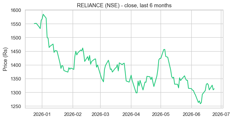
Load, then plot - the whole pipeline from a file to a finished chart of six months of Reliance, in a dozen lines. This load-analyse-visualise loop is the daily rhythm of working with market data.

Try it yourself

• Download a US stock with yf.Ticker("MSFT").history(period="1y"), save it with to_csv("msft.csv"), then read it back with read_csv.
• Open your saved reliance_6mo.csv in a plain text editor (or Excel). Confirm it really is just commas and numbers - nothing magic.
• Run df.describe() on the whole Reliance DataFrame (not just Close). Which column has the largest numbers, and why?

Recap

• Get a DataFrame from a download (yfinance) or a file (CSV) - the two everyday sources.
• df.to_csv("file.csv") saves; pd.read_csv("file.csv") loads - add index_col="Date" and parse_dates=True for time series.
• For Indian stocks on Yahoo, use the .NS suffix and .dropna() to drop incomplete bars.
• describe() gives an instant statistical summary - run it on every new dataset first.

We've quietly slipped a .dropna() into the last two chapters without dwelling on it. That's because real data is messy - missing values, wrong types, duplicates - and cleaning it is half the job. The next chapter tackles that head-on: data cleaning, with the genuine quirks of the data you just downloaded.