NumPy Basics

This is the module traders have been waiting for. Everything until now was learning the language; from here we put it to work on real market data. And the gateway tool is NumPy - the library that turns Python into a serious number-cruncher. You met it briefly in Chapter 1, where it ran a sum thirty times faster than plain Python. Now you'll wield it yourself. NumPy is the bedrock the entire data world stands on, so a solid hour here pays off for the rest of the course.

What is an array?

A NumPy array is like a list, but built for numbers and for speed. You create one by handing np.array a list of values - here, ten real recent closing prices for Apple:

import numpy as np

# 10 recent daily closes for AAPL (real data), stored as a NumPy array.
closes = np.array([291.58, 295.63, 291.13, 296.42, 299.24,
                   295.95, 298.01, 297.01, 294.30, 293.08])

print("Array     :", closes)
print("Count     :", closes.size)
print("Mean      :", round(closes.mean(), 2))   # stats are built right in
print("Std dev   :", round(closes.std(), 2))
print("Min / Max :", closes.min(), "/", closes.max())

Array     : [291.58 295.63 291.13 296.42 299.24 295.95 298.01 297.01 294.3  293.08]
Count     : 10
Mean      : 295.24
Std dev   : 2.54
Min / Max : 291.13 / 299.24

Two things already stand out. First, closes.mean() and closes.std() are built into the array - no sum/len gymnastics, just ask. Second, by convention NumPy is imported as np (that aliasing trick from Chapter 17), which you'll see in every data notebook on earth. An array knows it holds numbers, and that knowledge is what makes it fast.

Vectorised maths: the killer feature

Here's the idea that changes everything. With a list, doing maths on every element means writing a loop. With an array, you write one expression and it applies to the whole array at once - this is called vectorisation:

import numpy as np

closes = np.array([291.58, 295.63, 291.13, 296.42, 299.24,
                   295.95, 298.01, 297.01, 294.30, 293.08])

# Vectorised maths: one expression acts on the WHOLE array at once - no loop.
change = closes - closes[0]                # change vs day 1, for every day
print("Change vs day 1:", change.round(2))

# Daily percentage returns, for all days, in a single line.
returns = (closes[1:] - closes[:-1]) / closes[:-1] * 100
print("Daily returns %:", returns.round(2))
print("Average return :", round(returns.mean(), 3), "%")
print("Best day       :", round(returns.max(), 2), "%")

Change vs day 1: [ 0.    4.05 -0.45  4.84  7.66  4.37  6.43  5.43  2.72  1.5 ]
Daily returns %: [ 1.39 -1.52  1.82  0.95 -1.1   0.7  -0.34 -0.91 -0.41]
Average return : 0.063 %
Best day       : 1.82 %

The line (closes[1:] - closes[:-1]) / closes[:-1] * 100 computes every daily return in one go: "tomorrow's array minus today's array, over today's." No loop, and it reads like the formula itself. Once vectorised thinking clicks, you'll stop writing loops for number work entirely - and your code gets shorter and faster at the same time.

The thirty-times payoff

Remember the promise from Chapter 1? Here it is, now in your own hands - the same sum, the slow way and the NumPy way:

Copy

import time
from pathlib import Path

import matplotlib

matplotlib.use("Agg")
import matplotlib.pyplot as plt
import numpy as np
import seaborn as sns

N = 3_000_000

# Way 1: a plain Python loop - one number at a time.
t0 = time.perf_counter()
total = 0.0
for i in range(N):
    total += i * i
py_ms = (time.perf_counter() - t0) * 1000

# Way 2: NumPy - the same maths inside a compiled C core.
t0 = time.perf_counter()
arr = np.arange(N, dtype="float64")
total_np = (arr * arr).sum()
np_ms = (time.perf_counter() - t0) * 1000

speedup = py_ms / np_ms
print(f"Pure Python: {py_ms:8.1f} ms")
print(f"NumPy      : {np_ms:8.1f} ms")
print(f"Speed-up   : {speedup:.0f}x faster, same answer")

sns.set_theme(style="whitegrid")
fig, ax = plt.subplots(figsize=(6, 4))
ax.bar(["Pure Python", "NumPy (C core)"], [py_ms, np_ms], color=["#c98f8f", "#7c83ff"])
ax.set_ylabel("Time in milliseconds (lower is better)")
ax.set_title(f"Same sum, about {speedup:.0f}x faster with NumPy")
out = Path(__file__).with_suffix(".png")
plt.savefig(out, dpi=110, bbox_inches="tight")
print("Saved", out.name)

Live output

Pure Python:    285.8 ms
NumPy      :      8.0 ms
Speed-up   : 36x faster, same answer
Saved 03_speed.png

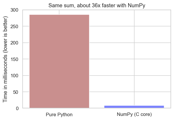
The bar says it all: the plain loop plods through millions of values one at a time; NumPy hands the whole job to its compiled C core and finishes in a flash. This array, and this vectorisation, is exactly what powered that headline number at the very start of the course.

Creating arrays without typing them

You rarely build big arrays by hand. NumPy has a family of constructors for the common shapes - a counting range, a block of zeros, evenly spaced points, even reproducible random numbers for simulations:

import numpy as np

# Handy ways to build arrays without typing every value.
print("arange(0,10,2) :", np.arange(0, 10, 2))      # start, stop, step
print("zeros(4)       :", np.zeros(4))               # all zeros
print("ones(3)        :", np.ones(3))                # all ones
print("full(3, 100)   :", np.full(3, 100))           # filled with one value
print("linspace(0,1,5):", np.linspace(0, 1, 5))      # 5 evenly spaced points

# Reproducible random numbers - e.g. simulated daily returns (seeded, so stable).
rng = np.random.default_rng(42)
print("random normals :", rng.normal(0, 1, 5).round(2))

# Reshape a flat array into rows and columns (a 2x3 grid).
grid = np.arange(6).reshape(2, 3)
print("reshaped 2x3   :\n", grid)

arange(0,10,2) : [0 2 4 6 8]
zeros(4)       : [0. 0. 0. 0.]
ones(3)        : [1. 1. 1.]
full(3, 100)   : [100 100 100]
linspace(0,1,5): [0.   0.25 0.5  0.75 1.  ]
random normals : [ 0.3  -1.04  0.75  0.94 -1.95]
reshaped 2x3   :
 [[0 1 2]
 [3 4 5]]

A few you'll reach for constantly: arange (like range, but an array), linspace (N evenly spaced points - great for axes), zeros/ones/full (pre-filled arrays), and reshape (turn a flat array into rows and columns). For simulations, np.random.default_rng(seed) gives a reproducible random generator - the same seeded idea from Chapter 18, now producing whole arrays of returns at once.

Dimensions: 1D, 2D and 3D arrays

An array can have more than one dimension. A 1D array is a single row of numbers (one stock's prices). A 2D array is a table - rows and columns (several stocks side by side). A 3D array is a stack of tables (say, the same table repeated over several weeks). Every array reports its shape (how big it is) and its ndim (how many dimensions):

import numpy as np

# 1D - a single row of values (one stock's prices).
oned = np.array([101.2, 103.5, 102.8])
print("1D:", oned, "| shape", oned.shape, "| ndim", oned.ndim)
print()

# 2D - a table: 3 days (rows) x 2 stocks (columns).
twod = np.array([
    [101.2, 250.1],
    [103.5, 248.7],
    [102.8, 252.3],
])
print("2D:\n", twod)
print("shape", twod.shape, "| ndim", twod.ndim)   # (3 rows, 2 columns)
print()

# 3D - a stack of tables (e.g. 2 weeks, each a 3-day x 2-stock table).
threed = np.arange(12).reshape(2, 3, 2)
print("3D shape:", threed.shape, "| ndim", threed.ndim)   # (2, 3, 2)

1D: [101.2 103.5 102.8] | shape (3,) | ndim 1

2D:
 [[101.2 250.1]
 [103.5 248.7]
 [102.8 252.3]]
shape (3, 2) | ndim 2

3D shape: (2, 3, 2) | ndim 3

Read .shape as (rows, columns): a (3, 2) array is 3 rows by 2 columns. You'll spend almost all your time in 1D (a price series) and 2D (a table of prices); 3D shows up occasionally - many stocks by many days by many fields - but it's the same idea with one more layer.

Slicing arrays

Slicing pulls a piece out of an array - and it's the exact same [start:stop] notation you learned for lists and strings in Chapter 8, just extended to more dimensions. In 2D you give two slices separated by a comma - [rows, columns] - and a bare : means "all of them":

import numpy as np

prices = np.array([
    [101.2, 250.1],   # day 0:  [stock A, stock B]
    [103.5, 248.7],   # day 1
    [102.8, 252.3],   # day 2
    [104.1, 255.0],   # day 3
])

# 1D slicing is exactly the list slicing from Chapter 8.
col_a = prices[:, 0]                       # every row, column 0 -> stock A's prices
print("Stock A (a column):", col_a)
print("First two of A    :", col_a[:2])    # plain [start:stop] slice

# 2D slicing: [rows, columns], separated by a comma. ":" means "all".
print("one cell [1, 0]   :", prices[1, 0])      # row 1, column 0
print("one row  [0, :]   :", prices[0, :])      # row 0, every column
print("one col  [:, 1]   :", prices[:, 1])      # every row, column 1
print("a block  [1:3, :] :\n", prices[1:3, :])  # rows 1-2, all columns

Stock A (a column): [101.2 103.5 102.8 104.1]
First two of A    : [101.2 103.5]
one cell [1, 0]   : 103.5
one row  [0, :]   : [101.2 250.1]
one col  [:, 1]   : [250.1 248.7 252.3 255. ]
a block  [1:3, :] :
 [[103.5 248.7]
 [102.8 252.3]]

The pattern to hold onto is array[rows, columns]. So prices[:, 0] reads "every row, column 0" - a whole column; prices[0, :] is "row 0, every column" - a whole row; and prices[1:3, :] is "rows 1 and 2, all columns" - a block. It really is just list slicing with a comma added for the second dimension.

Broadcasting: mixing different sizes

Here's the clever trick that makes vectorised maths so powerful. When you combine arrays of different sizes, NumPy automatically stretches the smaller one to fit. This is called broadcasting, and you've already used the simplest case - a single number applied to a whole array:

import numpy as np

prices = np.array([
    [101.2, 250.1],
    [103.5, 248.7],
    [102.8, 252.3],
])

# Scalar broadcasting: one number "stretches" to every element.
print("all prices + 1%:\n", (prices * 1.01).round(2))
print()

# Array broadcasting: a row of 2 values lines up with the 2 columns.
fee = np.array([0.5, 1.0])                 # a different fee per stock
print("minus a per-stock fee:\n", (prices - fee).round(2))
print()

# axis=0 works DOWN the columns: subtract each column's own mean (centre it).
col_means = prices.mean(axis=0)            # one mean per column
print("column means       :", col_means.round(2))
print("each value - its column mean:\n", (prices - col_means).round(2))

all prices + 1%:
 [[102.21 252.6 ]
 [104.54 251.19]
 [103.83 254.82]]

minus a per-stock fee:
 [[100.7 249.1]
 [103.  247.7]
 [102.3 251.3]]

column means       : [102.5  250.37]
each value - its column mean:
 [[-1.3  -0.27]
 [ 1.   -1.67]
 [ 0.3   1.93]]

Three things happened, each in one line. A single number (* 1.01) stretched to touch every element. A small row of two fees lined up with the two columns and applied to every row. And prices - prices.mean(axis=0) subtracted each column's own average from that whole column. That last line introduces axis: axis=0 runs down the rows (one result per column), while axis=1 runs across the columns (one result per row). Broadcasting is the reason you almost never write a loop - NumPy quietly works out how to line the shapes up for you.

Picking, aggregating and masking

Three everyday jobs - summarise an array, find where something is, and keep only what matches - each have a one-call answer:

import numpy as np

prices = np.array([101.2, 103.5, 99.8, 104.1, 98.5, 106.3])

# Aggregations collapse an array into a single answer.
print("sum     :", round(prices.sum(), 1))
print("cumsum  :", prices.cumsum().round(1))           # running total
print("argmax  :", prices.argmax(), "(index of the highest price)")
print("median  :", np.median(prices))
print("90th pct:", round(np.percentile(prices, 90), 2))

# Boolean masking - keep only the elements that pass a test.
print("above 100:", prices[prices > 100])
print("how many :", int((prices > 100).sum()))

# np.where picks between two values element by element.
labels = np.where(prices > 100, "up", "down")
print("labels   :", labels)

# np.diff = each value minus the previous one (day-to-day change).
print("diffs    :", np.diff(prices).round(1))

sum     : 613.4
cumsum  : [101.2 204.7 304.5 408.6 507.1 613.4]
argmax  : 5 (index of the highest price)
median  : 102.35
90th pct: 105.2
above 100: [101.2 103.5 104.1 106.3]
how many : 4
labels   : ['up' 'up' 'down' 'up' 'down' 'up']
diffs    : [ 2.3 -3.7  4.3 -5.6  7.8]

• Aggregations collapse an array to one number: sum, mean, std, median, np.percentile, and the running versions cumsum/cumprod.
• argmax/argmin give the position of the highest/lowest value (handy for "which day was the peak?").
• Boolean masking - prices[prices > 100] - keeps only the elements that pass a test, exactly the filtering idea you'll use all the time in pandas.
• np.where(condition, a, b) chooses between two values element by element - here labelling each day "up" or "down" in a single line.
• np.diff gives each value minus the previous one - day-to-day changes, the raw material of returns.

A NumPy cheat-sheet

You don't need to memorise these - just know they exist and look them up. The greatest hits, grouped by job:

• Create: np.array, np.arange, np.linspace, np.zeros, np.ones, np.full, np.random.default_rng().normal()
• Shape & dimensions: arr.shape, arr.ndim, arr.size, arr.reshape, arr.flatten, arr.T (transpose)
• Slice: arr[start:stop] (1D), arr[rows, cols] (2D), arr[:, 0] (a column), arr[0, :] (a row)
• Broadcasting & axis: arr * 2 / arr - row (auto-stretch), arr.mean(axis=0) (down columns), arr.sum(axis=1) (across rows)
• Maths (whole array): np.sqrt, np.log, np.exp, np.abs, np.round, np.clip (cap to a range), np.cumsum, np.cumprod, np.diff
• Summarise: sum, mean, std, var, min, max, median, np.percentile, argmax, argmin
• Logic & select: arr[arr > x] (mask), np.where, np.any, np.all, (arr > x).sum() (count matches)

That's the toolkit behind almost every calculation in quant finance - and pandas, which we meet next, is built directly on top of it.

Arrays vs lists

Both hold sequences, so when do you use which?

• A list is flexible: it can mix types (numbers, text, other lists) and is perfect for general-purpose collections - a watchlist of symbols, a stack of records.
• An array is specialised: all one numeric type, fixed in size, but vastly faster and able to do vectorised maths. Reach for it (and for pandas, which sits on top of it) whenever you're crunching numbers.

In practice you'll rarely create arrays by hand for real work - you'll get them from pandas, which loads market data into array-backed tables for you. But understanding the array underneath is what makes pandas make sense.

Try it yourself

• From the closes array, compute the array of prices expressed as a percentage of the first day: closes / closes[0] * 100.
• Find how many days closed above the average using (closes > closes.mean()).sum() - a neat vectorised counting trick.
• Build np.array([10, 20, 30, 40]) and, in one line each, double it, and subtract its own mean from every element.

Recap

• A NumPy array is a fast, numbers-only sequence created with np.array([...]) (imported as np).
• Vectorised maths applies one expression to the entire array at once - no loops - which is both clearer and far faster.
• Built-in stats (.mean(), .std(), .min(), .max()) come for free.
• Use lists for flexible, mixed collections; arrays (and pandas) for crunching numbers at speed.

NumPy gives you fast columns of numbers - but real market data has labels: dates, symbols, column names. The library that adds those labels on top of NumPy, and turns arrays into something that feels like a spreadsheet, is pandas. We start with its simplest piece, the Series, next.