Baskets and the Johansen Test

A pair trades just two stocks against each other, so you only estimate one number: the hedge ratio, how many units of one stock you hold against the other so their shared market moves cancel. But five bank stocks do not move in neat pairs. They are all dragged around by a single shared force - rates, the credit cycle, the banking factor. So the cleanest mean-reverting object hiding inside a sector is usually a basket: a weighted combination of three to five names, not a hand-picked twosome.

The promise of the basket is real. Pool the reversion across several legs, and no single bad quarter can snap the whole spread. But the cost is brutal, and badly advertised. Instead of one hedge ratio, you now estimate a whole vector of weights, one per stock. A vector fitted to a single window is a fragile, high-dimensional thing that overfits in ways a pair never could. This chapter builds the basket honestly with the Johansen test - the multi-stock version of a cointegration test, which finds stationary combinations among several stocks at once. Then it tears the basket down with its own out-of-sample numbers.

Why one pair is leaving information on the table

The Engle-Granger method handles exactly two series. You pick one as the dependent variable, regress, and test the leftover residual. That is a deliberate simplification, and it throws away structure. The five large-cap banks we use here - HDFCBANK, ICICIBANK, KOTAKBANK, AXISBANK, SBIN - share one dominant common factor. A pair of any two of them captures only a slice of that shared cycle. And the moment one name de-couples - a bad result, a regulatory action on a single bank - the two-leg spread breaks with nothing to cushion it. A basket spreads the bet across more legs, so a single name leaving the relationship does proportionally less damage.

We fix one estimation window for the whole chapter, 2019-01-01 to 2023-12-29 (1,239 trading days). We work in log prices throughout. Johansen, like Engle-Granger, is defined on I(1) levels, and a vector on logs reads as a unit-free, return-for-return relationship. Rebased to 100 at the window start, the five banks fan out and then wander back. The gap between the highest and lowest rebased line ranges from 0 to 137 index points across the window. That co-movement is necessary, but it is not enough on its own. The real question is whether a fixed combination of these prices is pinned to an average. Only a test can answer that.

What the Johansen test actually asks

Engle-Granger needs one series to play the left-hand side. With k names there is no natural choice, and there may be more than one stationary combination hiding inside the prices. The Johansen procedure treats all k series even-handedly. It fits a vector error-correction model and asks one question: of the k possible directions through these prices, how many are stationary rather than random walks? A stationary combination wanders around a fixed average and keeps getting pulled back to it. A random walk just drifts - each step is the last value plus noise, with no home to return to. The count of stationary directions is the cointegration rank, written r.

The eigenvectors that fall out of the procedure are the basket weights, ordered by how strongly each combination reverts. We run it with det_order=0 (a constant in the cointegrating relation, which suits drifting price levels) and one lag (k_ar_diff=1). Both are modelling choices we make, not defaults handed down from nature.

Running the test: trace and max-eigenvalue disagree

Johansen returns two sequences of statistics, each compared against tabulated 95% critical values. The trace statistic tests the hypothesis rank <= r against rank > r. You walk r up from zero and stop at the first rank you cannot reject. The maximum-eigenvalue statistic tests rank = r against rank = r+1, a sharper one-step-at-a-time test. On our basket, in this window, the two do not agree.

H0	trace stat	trace 95%	reject?	max-eig stat	max-eig 95%	reject?
rank <= 0	75.18	69.82	yes	29.61	33.88	no
rank <= 1	45.56	47.85	no	24.85	27.59	no
rank <= 2	20.72	29.80	no	14.61	21.13	no

The trace test clears its bar at rank <= 0 (75.18 > 69.82), then fails at rank <= 1 (45.56 < 47.85). So it picks rank r = 1: one stationary basket exists. The max-eigenvalue test never clears even its first bar (29.61 < 33.88). So it picks rank r = 0: no stationary combination at all. The two textbook statistics, run on identical data, return opposite verdicts.

Copy

fig, axes = plt.subplots(1, 2, figsize=(13, 4.8), sharex=True)
rs = np.arange(len(names))
for ax, stat, cv, ttl in [
    (axes[0], jr.lr1, jr.cvt[:, 1], 'Trace statistic vs 95% critical'),
    (axes[1], jr.lr2, jr.cvm[:, 1], 'Max-eigenvalue statistic vs 95% critical')]:
    cols = [C['green'] if s > c else C['grey'] for s, c in zip(stat, cv)]
    ax.bar(rs, stat, color=cols, width=0.62, label='test statistic')
    ax.plot(rs, cv, 'o--', color=C['red'], lw=1.6, ms=7, label='95% critical')
    for x, s, c in zip(rs, stat, cv):
        ax.text(x, s + 1.2, ('reject' if s > c else 'accept'), ha='center', fontsize=8.5,
                color=(C['green'] if s > c else C['grey']))
    ax.set_title(ttl); ax.set_xlabel('null hypothesis  rank <= r' if ax is axes[0] else 'rank r')
    ax.set_xticks(rs); ax.legend(fontsize=8.5)
axes[0].set_ylabel('statistic')
plt.tight_layout(); plt.show()
print(f'green bars (statistic above critical) = ranks we reject. trace -> r={r_trace}, maxeig -> r={r_maxeig}.')

Live output

green bars (statistic above critical) = ranks we reject. trace -> r=1, maxeig -> r=0.

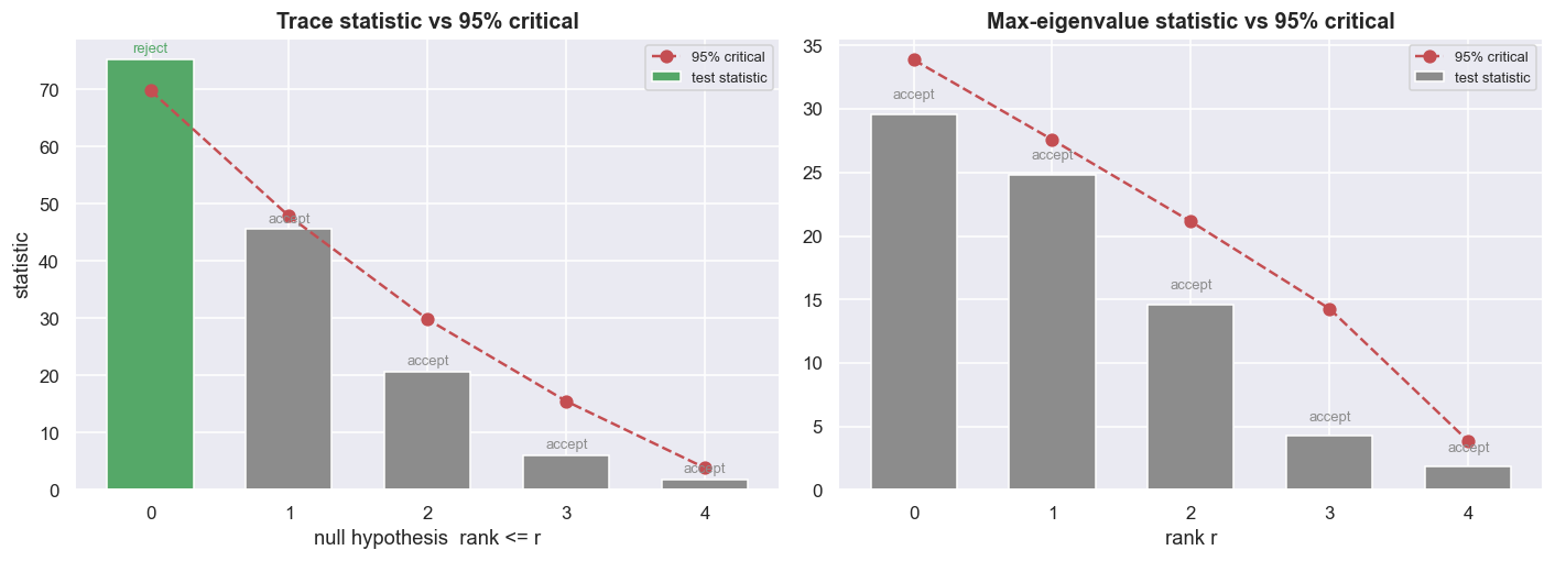
That disagreement is not a nuisance to smooth over. It is the finding. When trace and max-eigenvalue diverge, treat the rank evidence as contested, not settled - neither statistic is automatically right. The disciplined move is to fix your rule in advance, rather than pick the answer you prefer after seeing both. A sensible default is the more cautious reading (here the max-eigenvalue view), because it guards against reading too many relations into noise. Report both, and trade only the first eigenvector, if at all, and only after the basket survives out of sample. A weak, contested relationship is exactly the kind that fails to survive costs and regime change. The rest of the chapter shows that with numbers.

The cointegrating vector is your basket

The first column of the eigenvector matrix is the strongest-reverting combination. This set of weights is the cointegrating vector - the particular mix of the stocks that Johansen found to be stationary, and it doubles as your basket's portfolio weights. Its sign and scale are arbitrary, so we pin the first leg (HDFCBANK) to +1. The other weights then read as "per one unit long HDFCBANK, hold this much of each name."

Leg	Weight (HDFCBANK pinned to +1)	Side
HDFCBANK	+1.000	long
ICICIBANK	-0.166	short
KOTAKBANK	-0.518	short
AXISBANK	-0.115	short
SBIN	-0.017	short

So the basket is: long HDFCBANK against a weighted short of the other four, with KOTAKBANK carrying most of the short side. The basket spread is just vector . log-prices - the weighted sum of the prices that Johansen claims is stationary. We then take its z-score: how many standard deviations the spread sits from its own average right now, measured against the in-window mean and standard deviation. The spread crosses its mean 71 times across the window, the busy signature of reversion. The entry and exit bands at plus and minus one and two standard deviations are visible in the lower panel.

Copy

port = pd.Series(logpx.values @ v, index=logpx.index, name='basket')
mu, sd = port.mean(), port.std()
z = (port - mu) / sd

fig, (ax1, ax2) = plt.subplots(2, 1, figsize=(12, 7), sharex=True)
sns.lineplot(x=port.index, y=port.values, color=C['purple'], lw=1.1, ax=ax1)
ax1.axhline(mu, color=C['grey'], ls='--', lw=1.1, label='mean')
for k, cc in [(1, C['amber']), (2, C['red'])]:
    ax1.axhline(mu + k*sd, color=cc, ls=':', lw=1.0); ax1.axhline(mu - k*sd, color=cc, ls=':', lw=1.0)
ax1.fill_between(port.index, mu-sd, mu+sd, color=C['amber'], alpha=0.06)
ax1.set_title(f'Basket spread  =  vector . log-prices   ({WIN0[:4]}-{WIN1[:4]})'); ax1.set_ylabel('basket (log)')
ax1.legend(fontsize=8, loc='upper left')

sns.lineplot(x=z.index, y=z.values, color=C['blue'], lw=1.0, ax=ax2)
for k, cc in [(1, C['amber']), (2, C['red'])]:
    ax2.axhline(k, color=cc, ls=':', lw=1.0); ax2.axhline(-k, color=cc, ls=':', lw=1.0)
ax2.axhline(0, color=C['grey'], ls='--', lw=1.0)
ax2.fill_between(z.index, -1, 1, color=C['green'], alpha=0.05)
ax2.set_title('Basket z-score (entry/exit zones)'); ax2.set_ylabel('z'); ax2.set_xlabel('')
plt.tight_layout(); plt.show()

crossings = int((np.sign(z - 0).diff() != 0).sum())
print(f'mean crossings in-window: {crossings}  (a reverting basket crosses its mean often)')

Live output

mean crossings in-window: 71  (a reverting basket crosses its mean often)

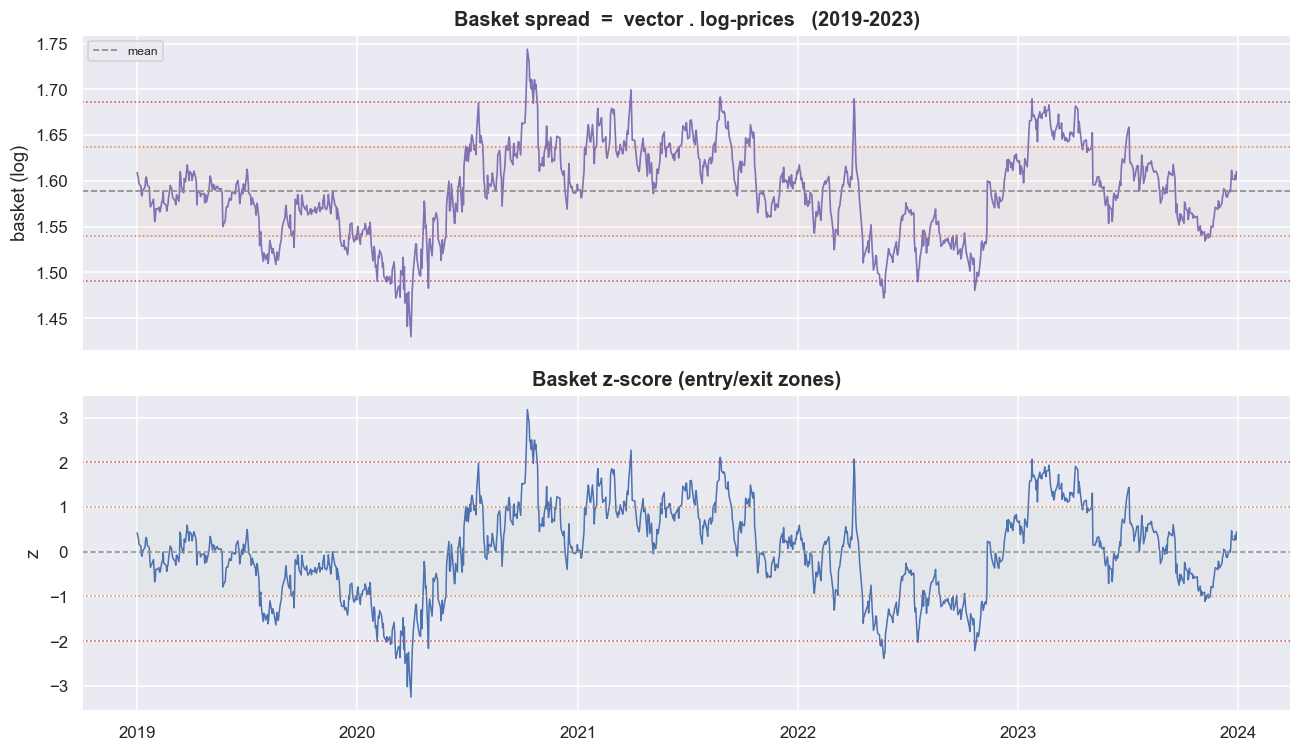
Now the formal test. The ADF test (Augmented Dickey-Fuller) asks whether a series is a random walk or genuinely mean-reverts. On the basket spread it gives a statistic of -4.285 and a p-value of 0.0005 (1%/5%/10% criticals -3.44 / -2.86 / -2.57). The p-value is the chance, if the spread really were a random walk, of seeing a result at least this extreme, so 0.0005 is a clean rejection of the random-walk case. The AR(1) half-life - how long a deviation takes to shrink by half, which is the natural holding period - is 23.7 trading days, about 1.1 months. The lag-1 autocorrelation of 0.971 is exactly what a 24-day half-life implies. On paper, this is a textbook mean-reverting basket.

Now the honesty: the vector will not hold still

Everything above is in-sample - measured on the same data we used to fit the vector. The single most dangerous assumption in basket trading is that the weight vector is a constant of nature. It is not. It is an estimate with k-1 free parameters, and it moves. Re-run Johansen on the first half and the second half of the same window, and the weights do not line up. They lurch.

Leg	full window	1st half	2nd half
ICICIBANK	-0.166	+0.621	-6.912
KOTAKBANK	-0.518	-1.250	-4.981
AXISBANK	-0.115	+0.581	-0.713
SBIN	-0.017	-0.797	+8.564

Three of the four free legs flip sign between the two halves. ICICIBANK goes from a long (+0.621) to a heavy short (-6.912). SBIN swings from -0.797 to +8.564. A sign flip is not a rounding wobble. It turns a long leg into a short one, which is catastrophic for any book holding the position. A block-bootstrap of the full-window vector confirms this is not just bad luck. The bootstrap standard deviation, measured against each weight's own size, is 1.43 for ICICIBANK, 1.07 for AXISBANK, and 1.84 for SBIN. When that ratio exceeds one, even the weight's sign is not reliably estimated.

Copy

def johansen_vec(df):
    j = coint_johansen(df.values, det_order=0, k_ar_diff=1)
    vv = j.evec[:, 0]; vv = vv / vv[0]      # normalise HDFCBANK = +1
    return pd.Series(vv, index=df.columns)

mid = logpx.index[len(logpx)//2]
vec_full = weights
vec_A = johansen_vec(logpx.loc[:mid])
vec_B = johansen_vec(logpx.loc[mid:])
comp = pd.DataFrame({'full window': vec_full, f'1st half': vec_A, f'2nd half': vec_B})
print(f'split at {mid.date()}')
print(comp.round(3).to_string())

longm = comp.reset_index().melt(id_vars='index', var_name='window', value_name='weight')
fig, ax = plt.subplots(figsize=(12, 4.8))
sns.barplot(data=longm, x='index', y='weight', hue='window',
            palette=[C['blue'], C['amber'], C['green']], ax=ax)
ax.axhline(0, color=C['grey'], lw=1.0)
ax.set_title('The "constant" cointegrating vector is not constant: same basket, two halves, different weights')
ax.set_ylabel('weight (HDFCBANK pinned to +1)'); ax.set_xlabel(''); ax.legend(title='', fontsize=9)
plt.tight_layout(); plt.show()
flip = ((np.sign(vec_A) != np.sign(vec_B)) & (vec_A.index != 'HDFCBANK')).sum()
print(f'legs whose SIGN flips between the two halves: {flip} of {len(names)-1} free legs  '
      f'-- a sign flip means long becomes short: catastrophic for a live book')

Live output

split at 2021-07-01
           full window  1st half  2nd half
HDFCBANK         1.000     1.000     1.000
ICICIBANK       -0.166     0.621    -6.912
KOTAKBANK       -0.518    -1.250    -4.981
AXISBANK        -0.115     0.581    -0.713
SBIN            -0.017    -0.797     8.564
legs whose SIGN flips between the two halves: 3 of 4 free legs  -- a sign flip means long becomes short: catastrophic for a live book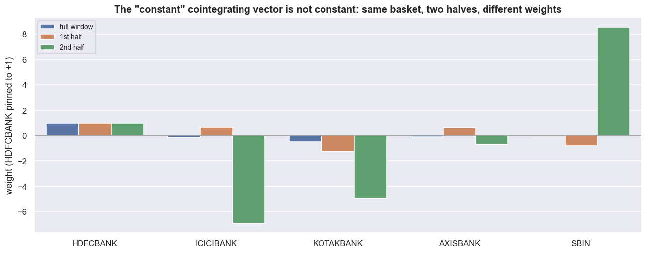

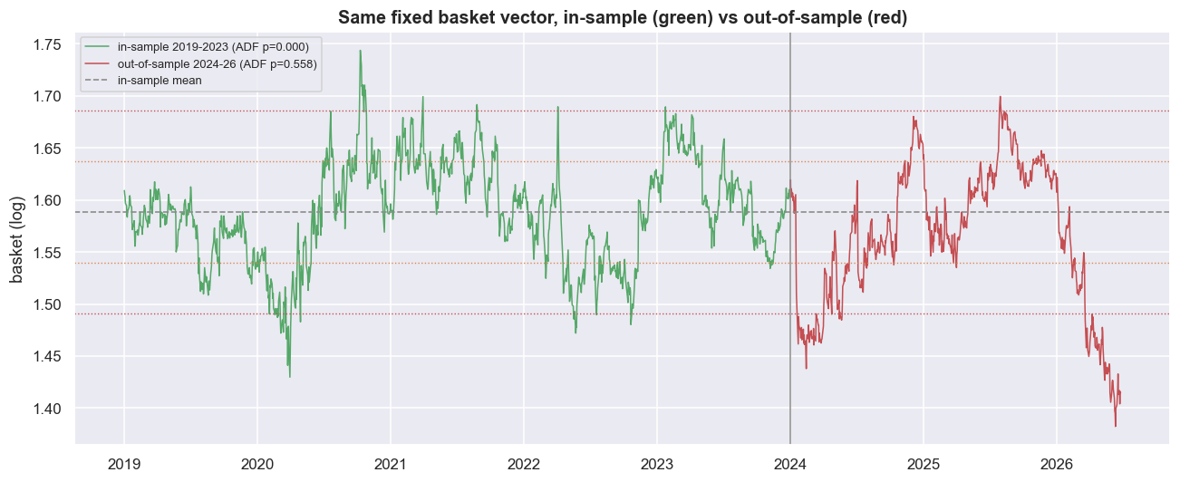
The cleanest way to show the damage is to take the vector fitted on 2019-2023 and apply it, unchanged, to 2024-2026 - data it never saw. That fresh, untouched data is the out-of-sample test, the only honest one. A genuinely cointegrated basket keeps reverting around the same average. This one does not. The out-of-sample spread drifts out of its bands, and the ADF p-value collapses from 0.0005 in-sample to 0.5583 out-of-sample - from "firmly stationary" to "cannot reject a random walk."

Copy

log_full = np.log(px_all).dropna()
port_full = pd.Series(log_full.values @ v, index=log_full.index)   # full-window IS vector, applied everywhere
is_part  = port_full.loc[WIN0:WIN1]
oos_part = port_full.loc['2024-01-01':]
adf_is  = adfuller(is_part,  autolag='AIC')[1]
adf_oos = adfuller(oos_part, autolag='AIC')[1]

fig, ax = plt.subplots(figsize=(12, 5))
ax.plot(is_part.index,  is_part.values,  color=C['green'], lw=1.0, label=f'in-sample {WIN0[:4]}-{WIN1[:4]} (ADF p={adf_is:.3f})')
ax.plot(oos_part.index, oos_part.values, color=C['red'],   lw=1.0, label=f'out-of-sample 2024-26 (ADF p={adf_oos:.3f})')
ax.axhline(mu, color=C['grey'], ls='--', lw=1.1, label='in-sample mean')
for k, cc in [(1, C['amber']), (2, C['red'])]:
    ax.axhline(mu + k*sd, color=cc, ls=':', lw=0.9); ax.axhline(mu - k*sd, color=cc, ls=':', lw=0.9)
ax.axvline(pd.Timestamp('2024-01-01'), color=C['grey'], lw=1.0)
ax.set_title('Same fixed basket vector, in-sample (green) vs out-of-sample (red)')
ax.set_ylabel('basket (log)'); ax.legend(fontsize=8.5, loc='upper left')
plt.tight_layout(); plt.show()
print(f'ADF p  in-sample {adf_is:.4f}  ->  out-of-sample {adf_oos:.4f}')
print('the relationship that looked airtight in-sample need not survive a regime it was not fitted on')

Live output

ADF p  in-sample 0.0005  ->  out-of-sample 0.5583
the relationship that looked airtight in-sample need not survive a regime it was not fitted on

This is structural, not unlucky. A k-leg vector has k-1 weights estimated from the same fixed sample. More legs means more parameters, which means more places for noise to creep in. And the bill is real. A one-way fill costs roughly 6.9 bps in our intraday cost model. So a two-leg pair round-trips at about 28 bps, while a five-leg basket round-trips at about 69 bps. Cost scales linearly with the number of legs, and a basket trips its threshold more often, because any single name can drag the spread across a band.

The selection trap: 94% in-sample, 0% out-of-sample

The deepest trap is the one nobody warns about. We are tempted not just to test a basket, but to pick the best one. List every sub-basket of 3, 4, and 5 of these banks - 16 combinations in all - and rank them by in-sample stationarity. The winners look spectacular. 94% of them test stationary in-sample at the 5% level. Now apply each winning vector, unchanged, to the out-of-sample window. Of those in-sample winners, 0% are still stationary out-of-sample. The in-sample and out-of-sample p-values carry a correlation of just +0.27 - close enough to nothing.

Copy

fig, ax = plt.subplots(figsize=(9.5, 6.2))
sns.scatterplot(data=sel, x='adf_p_IS', y='adf_p_OOS', hue='k', size='k',
                palette='viridis', sizes=(60, 160), ax=ax)
ax.axvline(0.05, color=C['green'], ls='--', lw=1.3); ax.axhline(0.05, color=C['green'], ls='--', lw=1.3)
ax.axhspan(0, 0.05, color=C['green'], alpha=0.05)
ax.text(0.052, 0.9, 'in-sample stationary -> ', color=C['green'], fontsize=9)
ax.text(0.5, 0.052, 'survives out-of-sample (the empty corner)', color=C['green'], fontsize=9)
ax.set_title('Basket selection overfits: in-sample stationarity does not carry out-of-sample')
ax.set_xlabel('ADF p-value  in-sample'); ax.set_ylabel('ADF p-value  out-of-sample')
ax.legend(title='legs', fontsize=8)
plt.tight_layout(); plt.show()
print('points hug the LEFT (great in-sample) but spread across the TOP (dead out-of-sample).')
print('the bottom-left "survives both" corner is nearly empty -- exactly the overfit we warned about.')

Live output

points hug the LEFT (great in-sample) but spread across the TOP (dead out-of-sample).
the bottom-left "survives both" corner is nearly empty -- exactly the overfit we warned about.

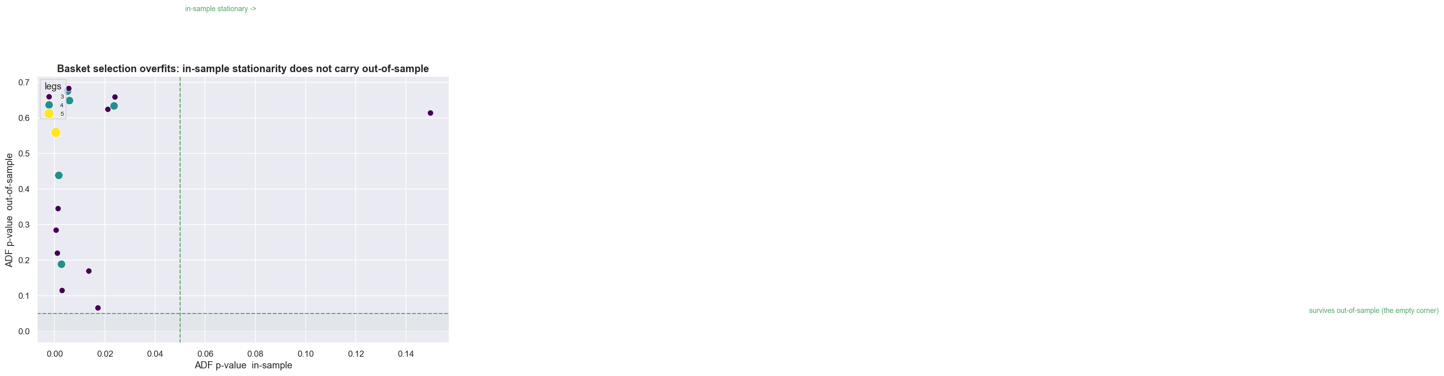
The strongest in-sample basket - the full five-name set, ADF p = 0.00047 - posts an out-of-sample p of 0.558. On the chart, the points hug the left edge (great in-sample) and smear across the top (dead out-of-sample). The bottom-left "survives both" corner is essentially empty. Picking the basket that tests best is look-ahead bias wearing a lab coat. The in-sample p-value tells you almost nothing about the future.

Where this breaks

Baskets buy you diversification of the mean-reversion bet, and surrender almost everything else to estimation error. Here are the failure modes, in rough order of how often each one kills a real basket:

• The cointegrating vector is unstable. Re-estimated on two halves of the same window, three of the four free weights flipped sign. A fixed vector is a snapshot of one regime, not a law. Any real implementation must re-estimate continuously, and pay the turnover (constant churn of the book) and overfitting that brings.
• Estimation error grows with the legs. With k-1 weights from one sample, the bootstrap standard deviation of several weights rivalled their own size, so even the sign was in doubt. Past a point, more legs means more noise, not more signal.
• Out-of-sample, the basket can simply stop reverting. The exact vector that gave an in-sample ADF p of 0.0005 drifted out of its bands and failed the test (p = 0.558) in the next window. In-sample stationarity is a weak hypothesis about the future.
• Selection is look-ahead by another name. 94% of sub-baskets looked cointegrated in-sample, and 0% survived out-of-sample, with the two p-values nearly uncorrelated. Picking "the basket that tests best" manufactures a result that does not exist.
• Trace and max-eigenvalue disagreed on the rank. When the two Johansen statistics diverge - r = 1 versus r = 0 here - the cointegration is weak. And weak cointegration is exactly what fails to survive costs and regime change.
• Every extra leg costs. Round-trip cost scales linearly with the number of legs (about 28 bps for a pair, 69 bps for a five-name basket), and a basket trips its threshold more often. The basket must out-earn the pair by a wide margin just to break even, and after costs it usually does not.

A basket is the right idea - pool the reversion, neutralise the common factor. But it is a dangerous object - a high-dimensional estimate that overfits. Treat the Johansen vector as a fragile prior, to be re-checked out-of-sample. Use the fewest legs that capture the relationship. And never trade the basket that simply won the in-sample scan. The next logical step is to stop hand-picking one basket at all. Instead, neutralise market and sector returns across the whole universe and rank the residuals - a cross-sectional, factor-neutral book.

Real-life implementation note. Everything here uses real equity price series to learn the statistics. Treat the short legs as a research abstraction unless you have a valid implementation path. In Indian markets a short may require stock futures, borrowed stock, intraday square-off, or another instrument, and each choice changes costs, margin, borrow availability, taxes, slippage, and risk. A statistical relationship existing is not the same as a tradable edge existing.