Dynamic Hedge Ratios with the Kalman Filter

A hedge ratio is how many units of one stock you trade against one unit of another, so their shared market moves cancel. A static hedge ratio fixes that number once and never moves it. The trouble is, the real relationship will not sit still. You fit one number - the slope of HDFCBANK on KOTAKBANK, say - on five years of data. From that moment you act as if it were a law of physics: 1.055 units of KOTAKBANK short for every unit of HDFCBANK long, in 2019 and still in 2026.

But two banks are not a law of physics. Their relative sensitivity shifts with rate cycles, loan books, index reweightings and sentiment. The moment that slope drifts, your "hedged" spread quietly stops being hedged. It leaks directional risk and breaches its own bands for reasons that have nothing to do with mean reversion. The obvious fix is a hedge ratio that updates every day. The Kalman filter is the elegant way to do it - a method that nudges the hedge ratio a little each day as new prices arrive, instead of fixing it once. This chapter builds one from scratch. Then, on the same real data, it shows you that the elegant thing lost the backtest to the dumb flat number. That result is the whole point.

The number that pretends to hold still

Start with the diagnostic that exposes the lie. OLS (ordinary least squares) is just the standard line of best fit, and we use it to estimate the hedge ratio. Instead of fitting one OLS line over the whole window, re-fit A = alpha + beta * B every single day, on a trailing 120-day window, using only past data. Then watch beta. If it sits still, the static number is defensible. If it wanders, the static spread is structurally mis-hedged.

Take HDFCBANK and KOTAKBANK over 2018-2026. The cointegration test actually picked this pair on the in-sample data - the stretch we use to build and tune the model - at p = 0.0306. So this is a real relationship, not a fabricated one. And the rolling beta is damning. The static in-sample fit hands you beta = 1.055. But the 120-day rolling beta over the same series ranges from -0.312 to +1.744, with a mean of 0.625 and a standard deviation of 0.413. Its full swing is 329% of its own mean, and it spends 7.5% of all days negative. Negative. For two banks. A negative hedge ratio says you should hedge one lender by going long the other - economic nonsense for two names that rise and fall together. So the static 1.055 is not a stable truth. It is the average of a quantity that genuinely moves.

But notice the trap on the right of that picture. The rolling beta confirms the static number is a fiction. It also shows that the naive fix is its own disease. A 120-day window is so jumpy that it manufactures hedge ratios no risk desk would ever trade, including the negative ones. What we actually want is something smoother than rolling OLS but still adaptive. That is exactly the gap a Kalman filter is built to fill.

A hidden state, estimated one bar at a time

Think of the hedge relationship as a hidden state. You never see it directly, and it drifts slowly over time. All you ever see is prices. The Kalman filter is built for exactly this situation. It estimates a hidden, slowly-moving state from noisy observations, one bar at a time, using only the past.

The state we track is the pair (intercept, hedge ratio), written x = [alpha, beta]. We assume it has no reason to move in any particular direction - only that it can wander. So we model it as a pure random walk: tomorrow's state is today's plus random noise, with no home value pulling it back. That is x_t = x_{t-1} + w, where w has covariance Q. The observation links today's price of A to the state and today's price of B: A_t = alpha_t + beta_t * B_t + v, with observation noise variance R. Then the filter runs two steps, forever:

The beautiful part is that the filter hands you the tradeable spread for free. The spread is what is left after you subtract one stock (scaled by the hedge ratio) from the other - it is the actual thing a pairs trade bets on. The innovation e_t = A_t - (alpha + beta * B_t) is the part of today's A that the filter did not expect from yesterday's state and today's B. That innovation is the dynamic spread. It uses only the past state plus today's B, so it is genuinely out-of-sample at every bar - it never peeks at data the model has not already seen. The Kalman gain K decides how much of each surprise to believe, and two knobs govern it entirely.

We set the process noise the Chan (2013) way, with a single dial delta: Q = delta / (1 - delta) * I. As delta -> 0, Q -> 0, and the state freezes into a static beta with extra steps. As delta grows, the state sprints and re-hedges on every wiggle. R is the skepticism dial. A large R says "most of today's move is noise, barely update." A small R says "lunge at every print." The key point: these two only ever matter as a ratio. A large Q/R trusts new data; a small Q/R trusts the prior.

We start with a deliberately ordinary choice, delta = 1e-4 and R = 1e-3. We stress-test it later.

Three betas on one axis

With those settings, the filter produces a beta that is everything we hoped for as a description. Over the full series its standard deviation is 0.087. That is smoother than rolling OLS by a factor of nearly five (rolling sd was 0.413). It ranges only from 0.635 to 1.067, and it never goes negative. It tracks genuine drift without the rolling estimate's nervous breakdowns.

Copy

fig, ax = plt.subplots(figsize=(12, 5.0))
ax.plot(rb.index, rb.values, color=C['grey'], lw=1.0, alpha=0.9, label='rolling 120d OLS beta (jumpy)')
ax.plot(kf.index, kf['beta'].values, color=C['teal'], lw=2.0, label=f'Kalman beta (delta={DELTA:.0e}, smooth)')
ax.axhline(beta_static, color=C['amber'], ls='--', lw=1.8, label=f'static IS OLS beta = {beta_static:.3f}')
ax.axhline(0, color=C['red'], lw=0.8, ls=':')
ax.axvspan(pd.Timestamp(OOS0), pd.Timestamp(OOS1), color=C['blue'], alpha=0.06, label='out-of-sample')
ax.set_title(f'Hedge ratio over time: static vs rolling-OLS vs Kalman   ({A_name} on {B_name})')
ax.set_ylabel('hedge ratio beta'); ax.legend(fontsize=8.5, ncol=2, loc='upper right')
plt.tight_layout(); plt.show()
print(f'The static line is flat at {beta_static:.3f}; the market spent most of the sample nearer '
      f'{kf["beta"].iloc[60:].median():.2f}. A single IS number can be wrong about the whole rest of the series.')

Live output

The static line is flat at 1.055; the market spent most of the sample nearer 0.73. A single IS number can be wrong about the whole rest of the series.

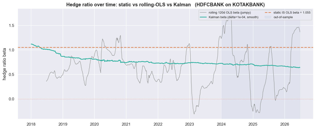
Look at where the lines sit. The static beta is pinned flat at 1.055. But the market spent most of the sample with a true ratio nearer 0.73. The Kalman line tracks down toward it, while the static line stays stubbornly high. As a picture of "what was the hedge ratio actually doing," the Kalman wins outright. The static line is a single in-sample number that is wrong about most of the rest of the series. If description were the goal, we would be done. It is not. The goal is P&L.

The dynamic spread you actually trade

We trade the Kalman spread with the identical machinery the static-beta backtest uses. The z-score measures how many standard deviations the spread sits from its own average right now - it is the entry and exit gauge. We standardise using a trailing 60-day rolling mean and standard deviation (no look-ahead), enter when |z| exceeds 2.0, and exit near 0.5. Keeping this machinery identical means the only thing that changes between the two backtests is the spread itself. That makes it a clean, single-variable comparison.

Copy

LOOKBACK, ENTRY, EXITZ = 60, 2.0, 0.5      # z-score window and trade thresholds (shared by both models)

def zscore(s, w=LOOKBACK):
    '''Trailing rolling z-score, no look-ahead (uses only the past w observations).'''
    return (s - s.rolling(w).mean()) / s.rolling(w).std()

spread_kal = kf['spread'].copy(); spread_kal.iloc[:60] = np.nan   # burn-in: drop unconverged start
z_kal      = zscore(spread_kal)
sqrtS      = np.sqrt(kf['S']);  sqrtS.iloc[:60] = np.nan

fig, (ax1, ax2) = plt.subplots(2, 1, figsize=(12, 7.4), sharex=True)
ax1.plot(spread_kal.index, spread_kal.values, color=C['purple'], lw=1.0, label='Kalman dynamic spread  e_t')
ax1.fill_between(sqrtS.index, -sqrtS.values, sqrtS.values, color=C['teal'], alpha=0.12,
                 label='+/- sqrt(S): filter uncertainty')
ax1.axhline(0, color=C['grey'], lw=0.9, ls='--')
ax1.axvspan(pd.Timestamp(OOS0), pd.Timestamp(OOS1), color=C['blue'], alpha=0.06)
ax1.set_title(f'Kalman dynamic spread and its z-score   ({A_name} - beta_t.{B_name})')
ax1.set_ylabel('forecast error (log)'); ax1.legend(fontsize=8.5, loc='upper left', ncol=2)

ax2.plot(z_kal.index, z_kal.values, color=C['blue'], lw=0.9)
for k, c, lbl in [(ENTRY, C['red'], f'+/- {ENTRY} entry'), (-ENTRY, C['red'], None),
                  (EXITZ, C['green'], f'+/- {EXITZ} exit'), (-EXITZ, C['green'], None)]:
    ax2.axhline(k, color=c, lw=1.1, ls=':' , label=lbl)
ax2.axhline(0, color=C['grey'], lw=0.8, ls='--')
ax2.fill_between(z_kal.index, ENTRY, z_kal.values, where=(z_kal.values>ENTRY), color=C['red'], alpha=0.25)
ax2.fill_between(z_kal.index, -ENTRY, z_kal.values, where=(z_kal.values<-ENTRY), color=C['red'], alpha=0.25)
ax2.axvspan(pd.Timestamp(OOS0), pd.Timestamp(OOS1), color=C['blue'], alpha=0.06)
ax2.set_ylabel(f'rolling z ({LOOKBACK}d)'); ax2.legend(fontsize=8.5, loc='upper left', ncol=3)
plt.tight_layout(); plt.show()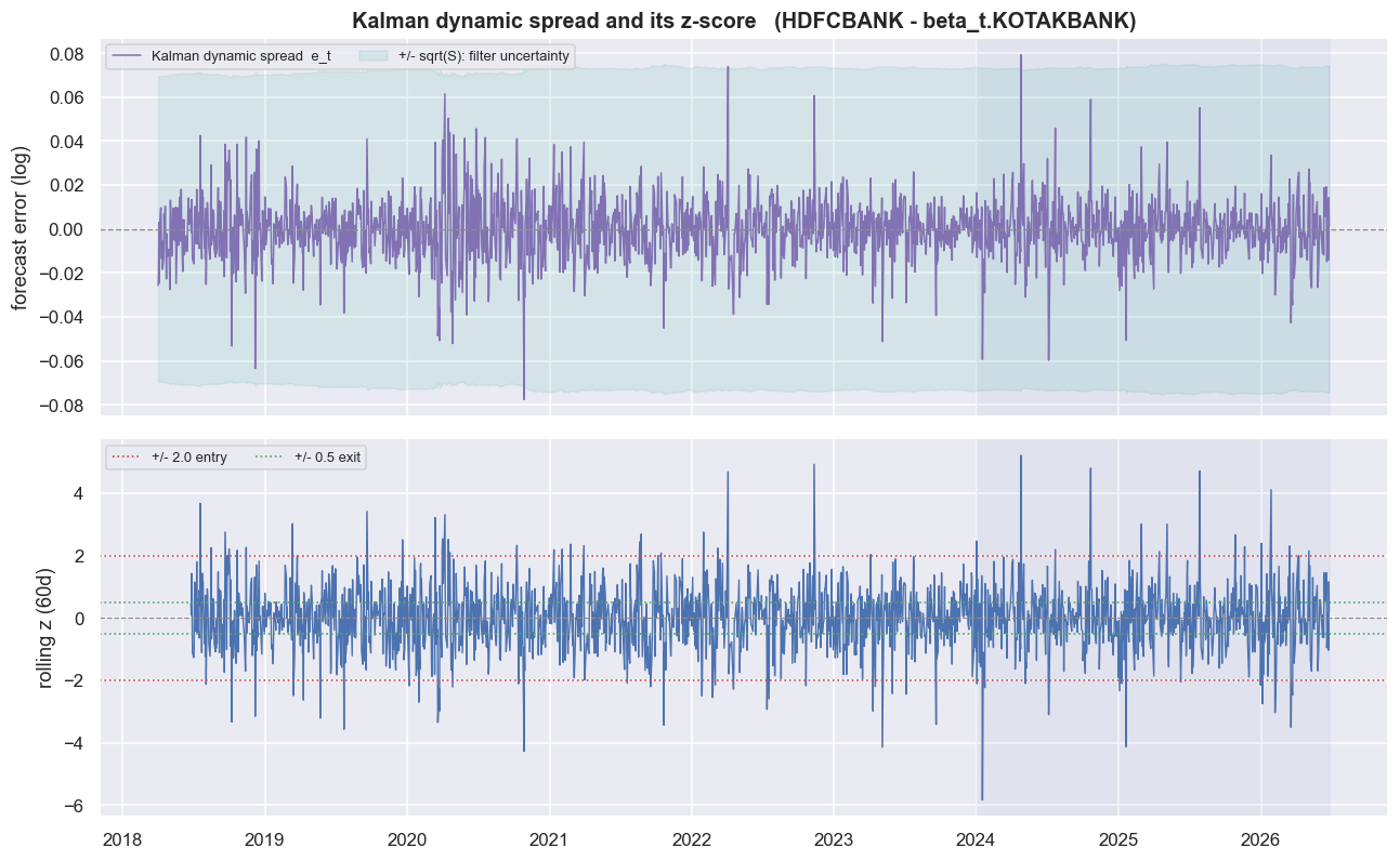

The top panel shows the dynamic spread with the filter's own +/- sqrt(S) uncertainty band. The bottom shows the rolling z-score crossing the entry and exit thresholds. It looks tradeable. It crosses zero, it stretches to the bands, and it comes back. Every visual instinct says this should work at least as well as the crude static spread. Now we let the cash flows vote.

The honest backtest: the simple beta wins

Same rules for both models, no cheating. The signal forms at the close, and the fill happens on the next bar (positions shifted one day). The beta used to size day t is the beta known at t, lagged into the P&L. Net results subtract a full round-trip cost on both legs every time the position changes, with the B-leg cost scaling by beta. Gross is before those costs; net is after; and stat arb lives or dies on net. And we always report in-sample and out-of-sample separately, because the in-sample curve is only a hypothesis and only the out-of-sample curve is evidence.

Copy

fig, axes = plt.subplots(1, 2, figsize=(13, 5.0), sharey=True)
for ax, (name, bt, col) in zip(axes, [('static beta', bt_static, C['amber']),
                                      ('Kalman beta', bt_kal, C['teal'])]):
    g = bt['gross'].cumsum(); n = bt['net'].cumsum()
    ax.plot(g.index, g.values, color=col, lw=1.8, label='gross')
    ax.plot(n.index, n.values, color=col, lw=1.6, ls='--', alpha=0.8, label='net of costs')
    ax.axhline(0, color=C['grey'], lw=0.8, ls=':')
    ax.axvspan(pd.Timestamp(OOS0), pd.Timestamp(OOS1), color=C['blue'], alpha=0.08, label='out-of-sample')
    shN_is,  _, _ = perf(bt['net'], IS0, IS1)
    shN_oos, _, _ = perf(bt['net'], OOS0, OOS1)
    ax.set_title(f'{name}\nnet Sharpe  IS {shN_is:+.2f}   OOS {shN_oos:+.2f}', fontsize=12)
    ax.set_ylabel('cumulative log return'); ax.legend(fontsize=9, loc='upper left')
fig.suptitle('Static vs Kalman: gross vs net, in-sample vs out-of-sample', fontweight='bold', y=1.02)
plt.tight_layout(); plt.show()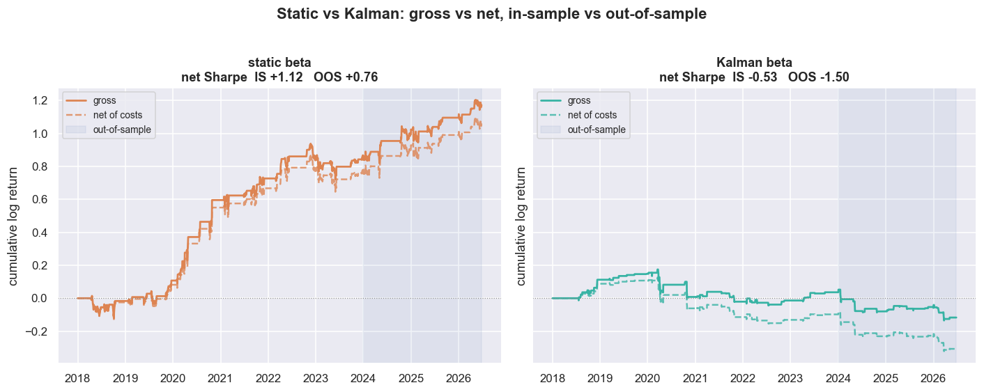

Here is the table the whole chapter has been walking toward. Net of costs:

Model	IS net Sharpe	OOS net Sharpe	Trades
Static beta	+1.12	+0.76	41
Kalman beta	-0.53	-1.50	78

The thing we spent two sections proving was "wrong" - the frozen 1.055 - earns a healthy +1.12 Sharpe in-sample. And the part that actually matters: it survives out-of-sample at +0.76 net. The Kalman beta, with all its adaptive sophistication and lovely smooth tracking, posts -0.53 in-sample and -1.50 out-of-sample. It also trades nearly twice as often (78 versus 41), paying costs on both legs each time, only to lock in a worse result. More flexibility did not buy more edge. It bought more ways to be wrong, plus a bigger commission bill for the privilege.

The knobs are a fit, not a discovery

A defender will say we just picked bad knobs - tune delta and R, and the Kalman will shine. So we tested that directly. We swept delta across two orders of magnitude at fixed R and watched the net out-of-sample Sharpe.

Copy

# sweep delta at fixed R; report IS and OOS net Sharpe, with the static result as the bar to beat
deltas = np.array([1e-6, 3e-6, 1e-5, 3e-5, 1e-4, 3e-4, 1e-3, 3e-3])
sweep = []
for d in deltas:
    kfd = kalman_hedge(A, B, delta=d, R=ROBS)
    spd = kfd['spread'].copy(); spd.iloc[:60] = np.nan
    btd = backtest(zscore(spd), kfd['beta'])
    sweep.append((d, perf(btd['net'], IS0, IS1)[0], perf(btd['net'], OOS0, OOS1)[0]))
sweep = pd.DataFrame(sweep, columns=['delta', 'IS_net_sharpe', 'OOS_net_sharpe'])

stat_is  = perf(bt_static['net'], IS0, IS1)[0]
stat_oos = perf(bt_static['net'], OOS0, OOS1)[0]

fig, ax = plt.subplots(figsize=(11, 4.8))
ax.plot(sweep['delta'], sweep['IS_net_sharpe'],  'o-', color=C['purple'], lw=1.8, label='Kalman IS net Sharpe')
ax.plot(sweep['delta'], sweep['OOS_net_sharpe'], 'o-', color=C['teal'],   lw=1.8, label='Kalman OOS net Sharpe')
ax.axhline(stat_is,  color=C['amber'], ls='--', lw=1.6, label=f'static IS net = {stat_is:+.2f}')
ax.axhline(stat_oos, color=C['red'],   ls='--', lw=1.6, label=f'static OOS net = {stat_oos:+.2f}')
ax.axhline(0, color=C['grey'], lw=0.8, ls=':')
ax.set_xscale('log'); ax.set_xlabel('delta  (process noise; bigger = faster-moving beta)')
ax.set_ylabel('annualised net Sharpe')
ax.set_title('Sensitivity to the process-noise knob: the Kalman result is a function of delta')
ax.legend(fontsize=8.5, ncol=2, loc='lower left')
plt.tight_layout(); plt.show()
disp = sweep.copy()
disp['delta'] = disp['delta'].map(lambda d: f'{d:.0e}')
disp['IS_net_sharpe'] = disp['IS_net_sharpe'].round(2)
disp['OOS_net_sharpe'] = disp['OOS_net_sharpe'].round(2)
print('Kalman net Sharpe by delta:'); print(disp.to_string(index=False))
print(f'\nNote: as delta -> 0 the Kalman freezes into the static beta and recovers toward it;')
print(f'as delta grows it chases noise and decays. No setting clears the static OOS bar of {stat_oos:+.2f}.')

Live output

Kalman net Sharpe by delta:
delta  IS_net_sharpe  OOS_net_sharpe
1e-06          -0.26           -0.12
3e-06          -0.50           -0.08
1e-05          -0.60           -0.84
3e-05          -0.76           -1.12
1e-04          -0.53           -1.50
3e-04          -0.87           -1.27
1e-03          -0.61           -1.05
3e-03          -0.55           -1.19

Note: as delta -> 0 the Kalman freezes into the static beta and recovers toward it;
as delta grows it chases noise and decays. No setting clears the static OOS bar of +0.76.

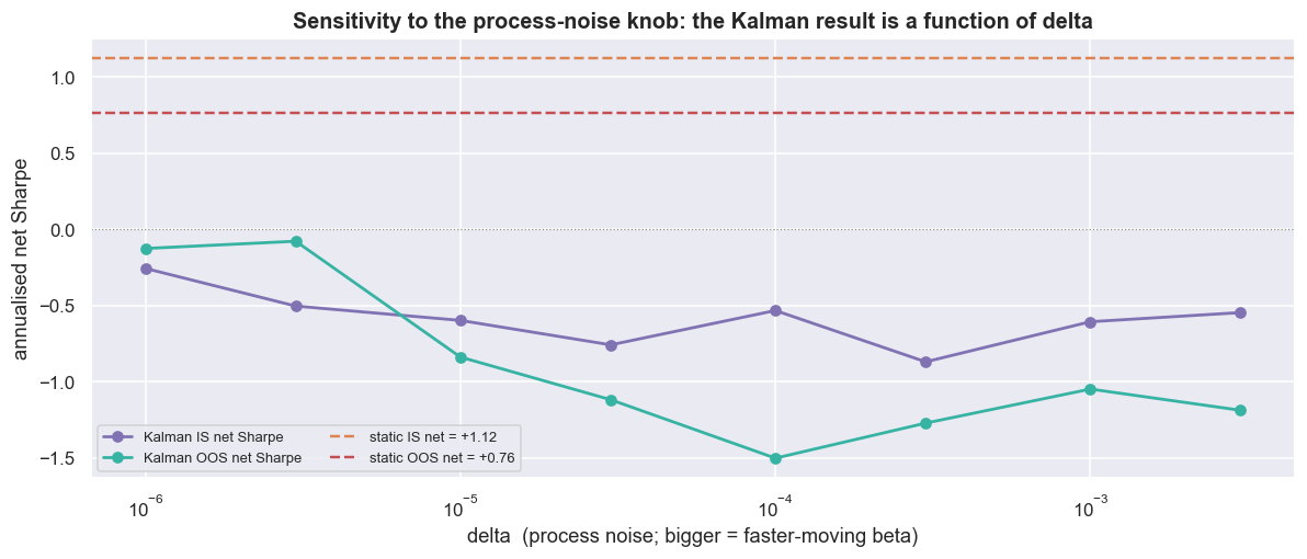
The OOS net Sharpe wanders from -0.08 at the gentlest setting down to -1.50, with no stable plateau. A tiny change in a knob we invented flips the result by more than a full Sharpe point. And here is the punchline: no value of delta clears the static OOS bar of +0.76. The best the Kalman manages is roughly break-even, at the very smallest delta. That is the filter quietly turning itself back into the static beta. The closer it gets to the static number, the better it does.

Then we ran the full two-dimensional delta x R grid, because what matters is the ratio, not either knob alone:

Copy

# the full Q x R surface: net OOS Sharpe over a grid of (delta, R)
d_grid = [1e-6, 1e-5, 1e-4, 5e-4, 1e-3]
r_grid = [1e-4, 1e-3, 1e-2, 1e-1]
grid = np.zeros((len(d_grid), len(r_grid)))
for i, d in enumerate(d_grid):
    for j, r in enumerate(r_grid):
        kfd = kalman_hedge(A, B, delta=d, R=r)
        spd = kfd['spread'].copy(); spd.iloc[:60] = np.nan
        btd = backtest(zscore(spd), kfd['beta'])
        grid[i, j] = perf(btd['net'], OOS0, OOS1)[0]
gridf = pd.DataFrame(grid, index=[f'{d:.0e}' for d in d_grid], columns=[f'{r:.0e}' for r in r_grid])

fig, ax = plt.subplots(figsize=(8.6, 5.4))
vmax = np.abs(grid).max()
sns.heatmap(gridf, annot=True, fmt='+.2f', cmap='vlag', center=0, vmin=-vmax, vmax=vmax,
            linewidths=0.5, cbar_kws={'label': 'net OOS Sharpe'}, ax=ax)
ax.set_xlabel('R  (observation noise)'); ax.set_ylabel('delta  (process noise)')
ax.set_title(f'Net OOS Sharpe across the Q x R tuning grid\n(static beta OOS net = {stat_oos:+.2f}; '
             f'grid spans {grid.min():+.2f} to {grid.max():+.2f})')
plt.tight_layout(); plt.show()
better = (grid > stat_oos).sum()
print(f'cells in the {grid.size}-point grid that beat the static OOS net Sharpe of {stat_oos:+.2f}: {better}')
print('The result is a landscape with hills and pits, not a number. Picking the best cell after the')
print('fact is curve-fitting; an honest forward test would have to fix delta and R *before* seeing OOS.')

Live output

cells in the 20-point grid that beat the static OOS net Sharpe of +0.76: 0
The result is a landscape with hills and pits, not a number. Picking the best cell after the
fact is curve-fitting; an honest forward test would have to fix delta and R *before* seeing OOS.

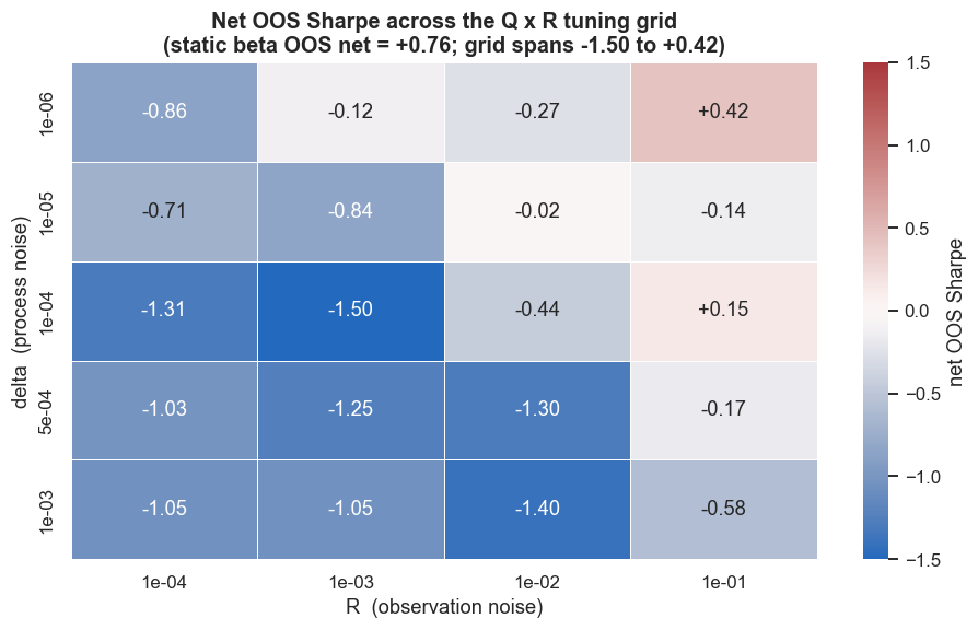
Of the 20 cells in the grid, the number that beat the static OOS net Sharpe of +0.76 is exactly 0. Not one. The surface is a landscape of hills and pits, not a single number. Picking the prettiest cell after seeing the out-of-sample result is curve-fitting, not edge. An honest forward test would have to fix delta and R before the OOS window exists. Any cell you fix on this evidence is a coin you already watched land heads.

Where this breaks

The Kalman filter is a genuinely better description of a drifting relationship than a static line. Whether it is a better trade is a separate question. And here, on a real cointegrated pair, in this window, net of costs, the answer was no. The ways it breaks:

• The tuning is a fit, full stop. delta and R have no market-given value. The grid swings the net OOS Sharpe across a wide range and sometimes flips its sign. Any single reported number is just one cell of an overfitting surface. The static beta has no such surface to get lost on.
• More flexibility, more ways to overfit. Every degree of freedom the Kalman adds is one more thing the in-sample optimiser can exploit. The price of adaptivity is a model that fits noise as eagerly as signal. And out-of-sample, noise does not repeat.
• A free intercept eats the very signal you trade. Letting alpha_t drift means the filter can quietly absorb a real, lasting mis-pricing into a "new mean," instead of flagging it as a deviation to fade. The dynamic spread can look mean-reverting on the chart while the tradeable edge has been filtered away into the moving intercept.
• The filter chases noise and pays for it twice. A larger delta re-hedges on day-to-day wiggle. That churns the book (78 trades versus 41), pays costs on both legs each time, and often locks in a worse beta just as the relationship wanders back. The net curve sits well below the gross curve for a reason.
• A dynamic hedge can still de-cointegrate. Tracking beta bar by bar does not guarantee the spread is stationary. An adaptive ratio can follow a relationship right out of its mean-reverting regime. That leaves you with a smooth, well-tracked, non-reverting series that is worse than useless.

Real-life implementation note. Everything here uses real adjusted equity closes to learn the statistics. The short leg is a research abstraction. Shorting one bank against the other in Indian markets needs a real vehicle (intraday square-off, borrowed stock, or a stock-futures proxy), and each choice changes costs, margin, borrow availability, taxes and slippage. A statistical relationship existing - even a Kalman-tracked one - is not the same as a tradable edge existing. On this pair, the most sophisticated estimator did not even win the research backtest, let alone the implementation one.