Risk, Sizing and Portfolio Construction

A single pair is a coin with a hidden bias and a habit of breaking. The previous chapters built one - HDFCBANK / KOTAKBANK - and then took it apart. Tested on fresh data it had never seen (out-of-sample), and after realistic costs, its Sharpe ratio was just 0.34 - return divided by risk, and a near-flat result. A beginner reacts by hunting for a better pair. A desk does the opposite. It stops betting everything on any one relationship and builds a portfolio - a basket of pairs where no single one can sink you. This chapter takes six same-sector pairs that look roughly cointegrated and does the real engineering. Neutralise the risks you do not want. Size each pair to a risk budget. Weight by risk instead of gut feel. And put hard safety rules underneath. The honest headline first: six pairs lift the out-of-sample net Sharpe (after costs) from 0.34 to 0.43, and shrink the worst drawdown - the deepest drop from a peak - from -13.8% to -10.0% in this data window. That is a steadier ride on the same thin edge, not a new edge. Everything that follows is about earning even that.

From one pair to a book that survives

We do not cherry-pick a winner. We take a broad list of same-sector candidates and re-estimate everything on the train window (2019-2023), exactly as before. Then we keep the six with the strongest sign of cointegration - where two prices each wander on their own, but a fixed combination of them stays tied together, as if by an invisible elastic band. We score that with the Engle-Granger test and keep the six lowest p-values (smaller means stronger evidence). We also require a tradeable half-life of 5 to 60 days - the half-life is how long a stretched spread takes, on average, to close half the gap back to its mean, which sets the natural holding period. The hedge ratio (how much of one stock you trade against the other), the trailing 60-day z-score (how many standard deviations the spread sits from its own average right now), and the next-bar fill are the same machinery as the single-pair notebooks. Nothing peeks at the future.

Pair	Sector	Train coint p	Hedge ratio	Half-life
M&M / MARUTI	Auto	0.0015	2.106	22.0
INFY / TCS	IT	0.0017	1.431	24.5
TCS / HCLTECH	IT	0.0217	0.682	21.3
HDFCBANK / KOTAKBANK	Banks	0.0306	1.054	29.3
TATASTEEL / JSWSTEEL	Metals	0.0356	1.052	45.9
HINDALCO / TATASTEEL	Metals	0.0686	0.820	38.9

Notice the flaw we left in on purpose. The two IT pairs both contain TCS, and the two metals pairs both contain TATASTEEL. Those pairs are not independent bets. When TCS is the short leg in one pair and the long leg in another, the two pairs move strongly opposite to each other. That is realistic. And it is the whole reason a book needs a covariance matrix - a grid that captures how every pair moves together with every other - and not just a list of each pair's own volatility (vol, the size of its typical swing).

The whole reason to bundle pairs is that they do not move together, so measure it. The average pairwise correlation of the six pairs' profits is just 0.04 - correlation runs from -1 to +1, and a value near 0 means almost no shared movement. The pairs are nearly independent. Each one earns in bursts and sits flat in between, and they do not all earn at the same time. That near-zero correlation is the engine that makes the whole book smoother than any single pair inside it.

Sizing: volatility targeting and the shrunk covariance

The six pairs are wildly unequal in risk. A one-unit M&M / MARUTI spread, with a hedge ratio above 2, swings several times more than a one-unit HDFCBANK / KOTAKBANK spread. Drop one raw unit of each into a book and M&M alone owns the risk - "diversification" becomes an empty word. Volatility targeting fixes this. The idea is simple: scale each pair so it contributes the same amount of risk. You multiply each pair by leverage = target_vol / its_own_vol, measured on the train window and then frozen, so every pair carries the same standalone risk (8% annualised). The leverages tell the story. M&M / MARUTI gets just 0.14 while TCS / HCLTECH gets 0.41 - the loudest pair is turned down the most.

Copy

TARGET_PAIR_VOL = 0.08
TARGET_PORT_VOL = 0.10

raw_vol = U.loc[TR0:TR1].std() * np.sqrt(ANN)        # standalone vol of each 1-unit spread (train)
lev     = TARGET_PAIR_VOL / raw_vol                  # constant per-pair leverage (frozen on train)
Rvt     = R.mul(lev, axis=1)                          # vol-targeted, signal-gated pair returns

# naive (one raw unit each) vs vol-targeted (equal risk), both scaled to the SAME 10% book vol
naive_pre = R.mean(axis=1)
vt_pre    = Rvt.mean(axis=1)
s_naive   = TARGET_PORT_VOL / (naive_pre.loc[TR0:TR1].std()*np.sqrt(ANN))
s_vt      = TARGET_PORT_VOL / (vt_pre.loc[TR0:TR1].std()*np.sqrt(ANN))
naive_bk  = naive_pre * s_naive
vt_bk     = vt_pre * s_vt

fig, axes = plt.subplots(1, 2, figsize=(13.5, 5.0), gridspec_kw=dict(width_ratios=[2, 3]))
ax = axes[0]
sns.barplot(x=raw_vol.values*100, y=raw_vol.index, hue=raw_vol.index, palette='flare', legend=False, ax=ax)
ax.axvline(TARGET_PAIR_VOL*100, color=C['green'], ls='--', lw=1.6)
ax.text(TARGET_PAIR_VOL*100, 5.4, f'  target {TARGET_PAIR_VOL*100:.0f}%', color=C['green'], fontsize=9)
ax.set_title('Standalone vol per 1-unit pair (train)'); ax.set_xlabel('annualized vol %'); ax.set_ylabel('')

ax = axes[1]
en, ev = eqc(naive_bk.loc[TR0:OO1]), eqc(vt_bk.loc[TR0:OO1])
pn, pv = perf(naive_bk.loc[TR0:OO1]), perf(vt_bk.loc[TR0:OO1])
ax.plot(en.index, en.values, color=C['grey'],  lw=1.8, label=f"naive (M&M dominates)  Sharpe {pn['sharpe']:.2f}")
ax.plot(ev.index, ev.values, color=C['green'], lw=2.0, label=f"vol-targeted (equal risk)  Sharpe {pv['sharpe']:.2f}")
ax.axvline(pd.Timestamp(OO0), color=C['grey'], ls='--', lw=1.0); ax.axhline(1, color=C['grey'], ls=':', lw=0.8)
ax.set_title(f'Naive vs vol-targeted book (both at {TARGET_PORT_VOL*100:.0f}% vol)')
ax.set_ylabel('growth of Rs 1'); ax.legend(fontsize=9, loc='upper left')
plt.tight_layout(); plt.show()

print('per-pair leverage (train):'); print(lev.round(2).to_string())
print(f"\nnaive book Sharpe {pn['sharpe']:.2f}  vs  vol-targeted {pv['sharpe']:.2f}   "
      f"(equalizing risk stops one pair owning the book)")

Live output

per-pair leverage (train):
M&M/MARUTI            0.14
INFY/TCS              0.28
TCS/HCLTECH           0.41
HDFCBANK/KOTAKBANK    0.33
TATASTEEL/JSWSTEEL    0.29
HINDALCO/TATASTEEL    0.29

naive book Sharpe 1.10  vs  vol-targeted 1.34   (equalizing risk stops one pair owning the book)

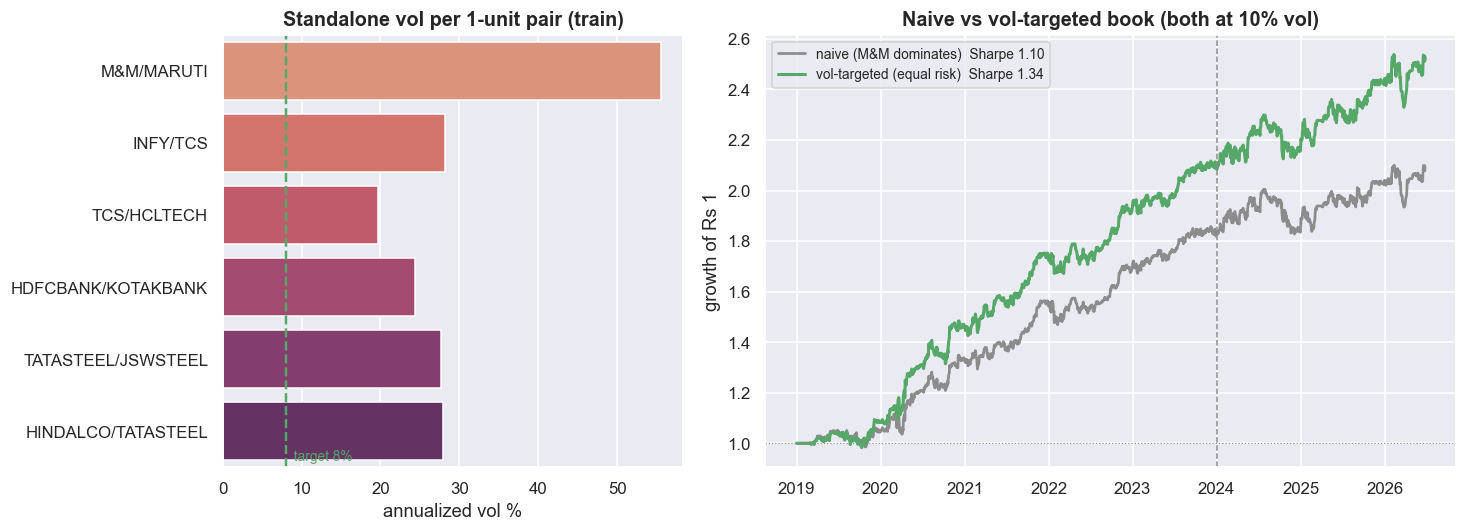
Equalising the risk lifts the book Sharpe from 1.10 (naive, one raw unit each) to 1.34 (vol-targeted). Both are scaled to the same 10% target, so the comparison is purely about balance, not about using more leverage. But vol targeting only fixes each pair's standalone risk. It is blind to how the pairs move together. That co-movement - driven by the shared legs - lives in the covariance matrix. And a covariance matrix has to be estimated from data, which is where the trouble starts.

Copy

from sklearn.covariance import LedoitWolf

Uvt   = U.mul(lev, axis=1)                     # always-on 1-unit spread returns, vol-targeted (equal diagonals)
Uvt_tr = Uvt.loc[TR0:TR1].fillna(0.0)         # diagonals ~equal, so what is left to estimate is the correlation
S_samp = Uvt_tr.cov().values
lwf    = LedoitWolf().fit(Uvt_tr.values)
S_lw   = lwf.covariance_
def corr_of(S):
    d = np.sqrt(np.diag(S)); return S / np.outer(d, d)

fig, axes = plt.subplots(1, 2, figsize=(13.5, 5.2))
for ax, M, ttl in [(axes[0], corr_of(S_samp), 'Sample correlation'),
                   (axes[1], corr_of(S_lw),  f'Ledoit-Wolf (shrinkage={lwf.shrinkage_:.2f})')]:
    sns.heatmap(M, ax=ax, xticklabels=BOOK, yticklabels=BOOK, annot=True, fmt='.2f',
                cmap='vlag', center=0, vmin=-1, vmax=1, cbar_kws=dict(label='corr'))
    ax.set_title(ttl); ax.tick_params(axis='x', rotation=90); ax.tick_params(axis='y', rotation=0)
plt.tight_layout(); plt.show()

# the honest test: condition number on SHORT rolling windows (what a desk re-estimates on)
cs, cl = [], []
for i in range(63, len(Uvt), 21):
    win = Uvt.iloc[i-63:i].fillna(0.0)
    try:
        cs.append(np.linalg.cond(win.cov().values))
        cl.append(np.linalg.cond(LedoitWolf().fit(win.values).covariance_))
    except Exception: pass
print(f'condition number, full train window : sample {np.linalg.cond(S_samp):5.1f}   Ledoit-Wolf {np.linalg.cond(S_lw):5.1f}')
print(f'condition number, 63-day windows med : sample {np.median(cs):5.1f}   Ledoit-Wolf {np.median(cl):5.1f}')
print(f'condition number, 63-day windows max : sample {np.max(cs):5.1f}   Ledoit-Wolf {np.max(cl):5.1f}')
print('higher condition number = closer to singular = the optimizer amplifies noise. Shrinkage keeps it tame.')

Live output

condition number, full train window : sample   4.7   Ledoit-Wolf   4.1
condition number, 63-day windows med : sample   6.9   Ledoit-Wolf   2.3
condition number, 63-day windows max : sample  16.7   Ledoit-Wolf   8.2
higher condition number = closer to singular = the optimizer amplifies noise. Shrinkage keeps it tame.

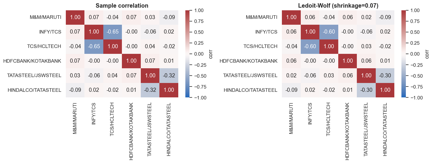
With six pairs and a short window, the measured covariance is noisy and unstable. Feed such a matrix to an optimiser and it produces garbage weights, because it blows up tiny measurement errors in the most unstable directions. The way to measure that instability is the condition number (the ratio of the largest to the smallest eigenvalue; higher means more unstable). On the realistic 63-day windows a desk actually re-estimates on, the raw sample matrix has a median condition number of 6.9 (max 16.7). Covariance shrinkage pulls those noisy estimates toward a simpler, steadier target - the Ledoit-Wolf method is the standard recipe. It cuts the condition number to 2.3 (max 8.2) - roughly a 3x gain in stability, trading a little bias for a lot of steadiness. The heatmaps make the shared legs visible: the two IT pairs sit at a strong negative correlation through TCS, the metals pairs through TATASTEEL.

Weighting by risk, not by gut

With a trustworthy covariance you can weight the pairs by risk. Here are two classic schemes, both long-only, with weights that add up to one, and both under a hard concentration cap of 35% so no single pair can take over. Minimum variance puts weight where it lowers the book's total swing the most - it loves the negatively-correlated IT pair that hedges its sibling. Risk parity, also called equal risk contribution (ERC), sizes things so every pair supplies the same share of the book's volatility. Minimum variance gives the lowest model vol by design (2.55% versus 2.77% for equal weight). ERC sits a touch higher at 2.60%, buying balance for a sliver of extra variance. ERC matters because equal money in each pair is not the same as equal risk from each pair.

Copy

rc_eq = risk_contrib(w_eq, S_lw) * 100
rc_rp = risk_contrib(w_rp, S_lw) * 100
rcdf  = pd.DataFrame({'equal-weight': rc_eq, 'risk-parity (ERC)': rc_rp}, index=BOOK)

fig, ax = plt.subplots(figsize=(12, 4.8))
rcdf.plot(kind='bar', ax=ax, color=[C['grey'], C['green']], width=0.78)
ax.axhline(100/6, color=C['amber'], ls='--', lw=1.4, label='equal share (1/6 = 16.7%)')
ax.set_title('Risk contribution to book volatility: equal capital is NOT equal risk')
ax.set_ylabel('% of book risk'); ax.set_xticklabels(BOOK, rotation=25, ha='right', fontsize=9); ax.legend(fontsize=9)
plt.tight_layout(); plt.show()

print('equal-weight risk contributions (%):', np.round(rc_eq, 1))
print('risk-parity  risk contributions (%):', np.round(rc_rp, 1), ' <- equalized by construction')

Live output

equal-weight risk contributions (%): [23.7  9.7  8.6 26.  17.7 14.4]
risk-parity  risk contributions (%): [16.7 16.7 16.7 16.7 16.7 16.7]  <- equalized by construction

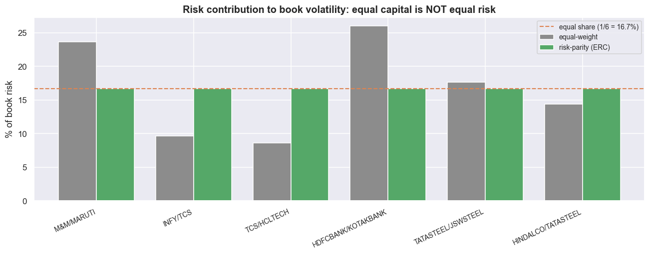
Under naive equal weighting the risk is lopsided. HDFCBANK / KOTAKBANK supplies 26.0% of the book's volatility and M&M / MARUTI 23.7%, while the two IT pairs supply only 9.7% and 8.6%. Two pairs out of six carry half the risk. After vol targeting, each pair's standalone risk is roughly equal, so this imbalance comes almost entirely from the correlations. The IT pairs hedge each other and add little net risk, while the standalone bank and auto pairs add a lot. Risk parity flattens every contribution to exactly 16.7% (1/6). The concentration cap is the backstop underneath: no pair holds more than 35% of capital, so one broken pair can never sink the book alone.

Rupee-neutral is not beta-neutral

Now the exposures. A long/short book has two size numbers. Gross exposure is the sum of the legs ignoring sign - what you actually trade, pay costs on, and post margin against. Net exposure is the signed sum - your leftover directional tilt. Gross rises and falls with how many pairs are firing (mean 1.08x, peaking at 2.80x), while net stays near zero (mean +0.017x), because every pair is long one stock and short another. That looks market-neutral. It is not. "Equal money long and short" is rupee-neutral. "Equal market sensitivity long and short" is beta-neutral. The two come apart the moment the two legs have different betas to NIFTY. A pair's beta is beta_A - hedge_ratio x beta_B, so a large hedge ratio magnifies any mismatch.

Copy

rnif = nifty.pct_change()
def mkt_beta(rs):
    x = pd.concat([rs, rnif], axis=1).loc[TR0:TR1].dropna()
    return np.cov(x.iloc[:,0], x.iloc[:,1])[0,1] / np.var(x.iloc[:,1])

legbeta = {}
for k in BOOK:
    legbeta[allp[k]['a']] = mkt_beta(px[allp[k]['a']].pct_change())
    legbeta[allp[k]['b']] = mkt_beta(px[allp[k]['b']].pct_change())
# market beta of one long-spread unit = beta_A - hedge_ratio * beta_B
pair_mbeta = {k: legbeta[allp[k]['a']] - beta[k]*legbeta[allp[k]['b']] for k in BOOK}

# time-varying book beta (sum over active pairs), and the NIFTY overlay that neutralizes it
book_beta   = sum(exposure[k] * Hd[k] * pair_mbeta[k] for k in BOOK)
book_hedged = book_net + (-book_beta.shift(1).fillna(0.0)) * rnif     # short the residual beta in NIFTY
def roll_beta(r, w=120):
    d = pd.concat([r, rnif], axis=1).dropna()
    return (d.iloc[:,0].rolling(w).cov(d.iloc[:,1]) / d.iloc[:,1].rolling(w).var())
rb_before, rb_after = roll_beta(book_net), roll_beta(book_hedged)

fig, axes = plt.subplots(1, 2, figsize=(13.5, 5.0), gridspec_kw=dict(width_ratios=[2,3]))
ax = axes[0]
mb = pd.Series(pair_mbeta).reindex(BOOK)
sns.barplot(x=mb.values, y=mb.index, hue=mb.index, palette='vlag', legend=False, ax=ax)
ax.axvline(0, color=C['grey'], lw=1.0)
ax.set_title('Market beta of each 1-unit pair\n(rupee-neutral does NOT mean beta-neutral)')
ax.set_xlabel('beta to NIFTY'); ax.set_ylabel('')
ax = axes[1]
ax.plot(rb_before.index, rb_before.values, color=C['red'],  lw=1.4, label=f'book beta, unhedged (mean {rb_before.mean():+.2f})')
ax.plot(rb_after.index,  rb_after.values,  color=C['green'], lw=1.4, label=f'book beta, NIFTY-overlay hedged (mean {rb_after.mean():+.2f})')
ax.axhline(0, color=C['grey'], ls='--', lw=0.9)
ax.set_title('Realized rolling 120-day beta of the book to NIFTY')
ax.set_ylabel('rolling beta'); ax.legend(fontsize=9, loc='upper left')
plt.tight_layout(); plt.show()

print('pair market betas:', {k: round(v,2) for k,v in pair_mbeta.items()})
print(f'book beta(t): mean {book_beta.mean():+.3f}  sd {book_beta.std():.3f}  peak |{book_beta.abs().max():.2f}|  '
      f'-> a "market-neutral" book can quietly carry market risk when a high-hedge-ratio pair is on.')

Live output

pair market betas: {'M&M/MARUTI': np.float64(-1.11), 'INFY/TCS': np.float64(-0.17), 'TCS/HCLTECH': np.float64(0.19), 'HDFCBANK/KOTAKBANK': np.float64(-0.02), 'TATASTEEL/JSWSTEEL': np.float64(-0.0), 'HINDALCO/TATASTEEL': np.float64(0.27)}
book beta(t): mean +0.008  sd 0.095  peak |0.28|  -> a "market-neutral" book can quietly carry market risk when a high-hedge-ratio pair is on.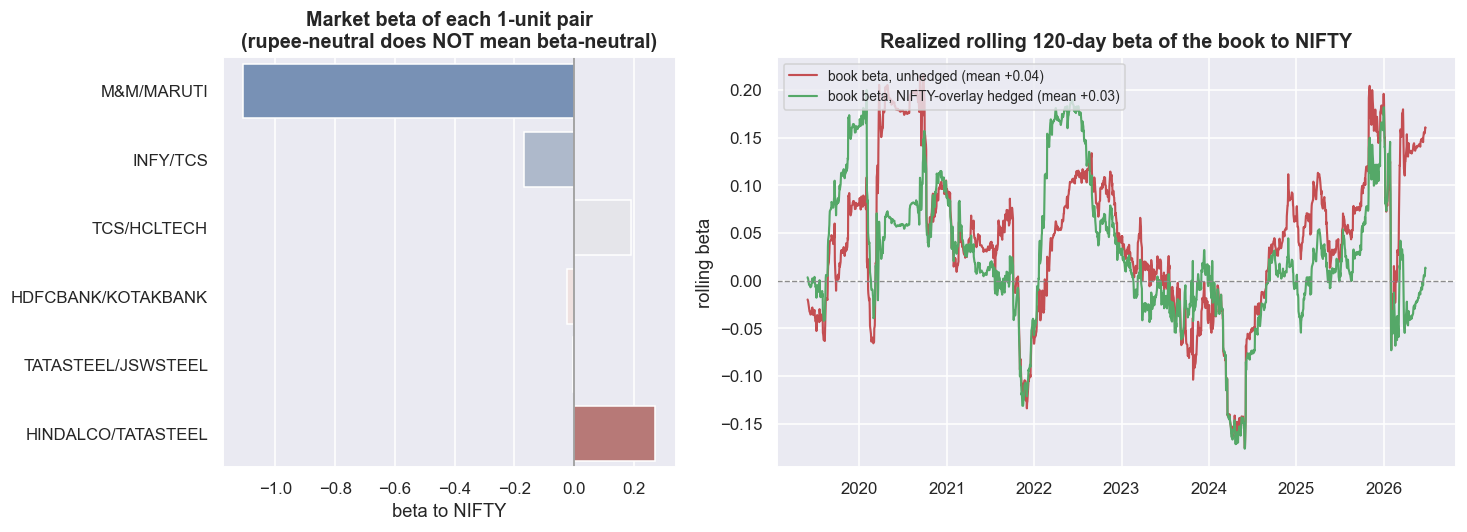

M&M / MARUTI is the cautionary tale. Its pair beta to NIFTY is -1.11, while every other pair sits between -0.17 and +0.27. Add up the betas across the active pairs and the book's leftover beta has a mean of just +0.008, but a standard deviation of 0.095 and peaks at |0.28|. So a "market-neutral" book quietly carries a quarter-unit of market risk whenever that high-hedge-ratio pair is on. The fix is a NIFTY overlay: each day, take a small offsetting position in the index equal to yesterday's leftover beta, and the realised rolling 120-day beta drops toward zero. Sector neutrality is cleaner by design, because every pair lives inside a single sector, so the net tilts stay tiny next to the gross (IT: 0.464 gross, 0.019 net; Metals: 0.372 gross, -0.003 net). The metals pairs sharing TATASTEEL are where a small net tilt can still leak in.

Put it all together - vol-targeted returns, risk-parity weights, scaled to 10% portfolio vol, and charged realistic delivery (CNC) costs of about 47 bps per leg-notional on every position change - and the full-sample net Sharpe is 0.94. Out of sample it is 0.43, total +9.0%, max drawdown -10.0%. Steadier than the single pair, but the out-of-sample haircut is the same hard fact it always was.

The stop-loss-on-a-spread dilemma

On a single stock, a stop-loss is plain risk control. On a mean-reverting spread it is a paradox. A spread stretched to |z| > 3 is, by the strategy's own logic, more likely to revert - so the stop fires exactly when the expected payoff from waiting is highest. Cut the position and you lock in a loss right before the snap-back. Hold it and a pair that has genuinely broken can run against you with no limit. This is not a tuning problem. It is built into the trade.

Copy

# find the most painful REAL stop in the book (excluding the COVID crash, a genuine break),
# where the stop fired and the spread then reverted hard -- the dilemma made concrete.
COVID = (pd.Timestamp('2020-02-15'), pd.Timestamp('2020-05-31'))
best = None
for k in BOOK:
    z, unit = allp[k]['z'], allp[k]['unit']; held = positions(z)
    for i in range(1, len(z)-1):
        if held.iloc[i] == 0 and held.iloc[i-1] != 0 and abs(z.iloc[i]) > STOP:
            if COVID[0] <= z.index[i] <= COVID[1]: continue
            j = i-1
            while j > 0 and held.iloc[j-1] == held.iloc[i-1]: j -= 1
            dirn = held.iloc[i-1]
            kk = i
            while kk < len(z)-1 and abs(z.iloc[kk]) > EXIT and kk-i < 60: kk += 1
            pnl_stop = float((dirn*unit.iloc[j+1:i+1]).sum())
            pnl_hold = float((dirn*unit.iloc[j+1:kk+1]).sum())
            if kk-i >= 3 and (best is None or pnl_hold-pnl_stop > best['regret']):
                best = dict(pair=k, e=z.index[j], s=z.index[i], r=z.index[kk],
                            pnl_stop=pnl_stop, pnl_hold=pnl_hold, regret=pnl_hold-pnl_stop, dirn=int(dirn))

k = best['pair']; z = allp[k]['z']; sp = (np.log(px[allp[k]['a']]) - beta[k]*np.log(px[allp[k]['b']]))
lo, hi = best['e'] - pd.Timedelta(days=20), best['r'] + pd.Timedelta(days=20)
zw = z.loc[lo:hi]
fig, (ax1, ax2) = plt.subplots(2, 1, figsize=(12.5, 7.0), sharex=True, gridspec_kw=dict(height_ratios=[1,1.2]))
ax1.plot(sp.loc[lo:hi].index, sp.loc[lo:hi].values, color=C['purple'], lw=1.5)
ax1.set_title(f"Stop-loss dilemma on {k}: spread (log)"); ax1.set_ylabel('spread')
for d, c, lab in [(best['e'], C['amber'], 'entry'), (best['s'], C['red'], 'STOP fires'), (best['r'], C['green'], 'reverts to mean')]:
    ax1.axvline(d, color=c, ls='--', lw=1.4); ax1.text(d, sp.loc[lo:hi].max(), '  '+lab, color=c, fontsize=9, va='top')
ax2.plot(zw.index, zw.values, color=C['blue'], lw=1.5)
ax2.axhline(STOP*np.sign(best['dirn']*-1), color=C['red'], ls='--', lw=1.2, label=f'stop (|z|={STOP})')
ax2.axhline(0, color=C['grey'], ls='--', lw=0.8); ax2.axhline(-EXIT*np.sign(best['dirn']*-1), color=C['green'], ls=':', lw=1.0, label='exit band')
for d, c in [(best['e'], C['amber']), (best['s'], C['red']), (best['r'], C['green'])]:
    ax2.axvline(d, color=c, ls='--', lw=1.4)
ax2.set_title('z-score: the stop fired at the extreme, then the spread came home'); ax2.set_ylabel('z'); ax2.legend(fontsize=9, loc='upper right')
plt.tight_layout(); plt.show()

print(f"trade: {k}, {('short' if best['dirn']<0 else 'long')} the spread, entered {best['e'].date()}")
print(f"  STOPPED OUT on {best['s'].date()} for {best['pnl_stop']*100:+.1f}%  (1-unit spread P&L)")
print(f"  had we HELD to the reversion on {best['r'].date()}: {best['pnl_hold']*100:+.1f}%")
print(f"  the stop cost {best['regret']*100:.1f}% of missed reversion -- and yet, on a pair that truly breaks,")
print(f"  that same stop is the only thing standing between you and an unbounded loss. That is the dilemma.")

Live output

trade: HDFCBANK/KOTAKBANK, short the spread, entered 2020-10-07
  STOPPED OUT on 2020-10-09 for -6.4%  (1-unit spread P&L)
  had we HELD to the reversion on 2021-01-05: +21.4%
  the stop cost 27.9% of missed reversion -- and yet, on a pair that truly breaks,
  that same stop is the only thing standing between you and an unbounded loss. That is the dilemma.

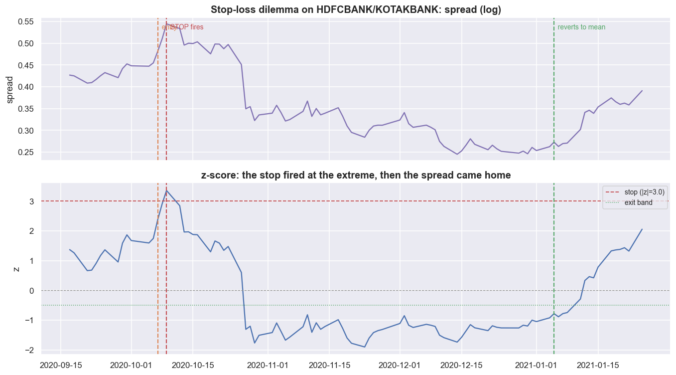
The most painful real example in this book (leaving out the COVID crash, which was a genuine break) is concrete. HDFCBANK / KOTAKBANK, short the spread, entered 2020-10-07, stopped out two days later on 2020-10-09 for -6.4%. Had you held on, the spread reverted to its mean by 2021-01-05 for +21.4%. The stop did not save you. It cost 27.9% of the missed reversion, cutting at the worst possible moment.

The same tension runs through drawdown control. Here is a simple throttle that only uses past data: cut the book's exposure to half once it falls 5% below its previous peak (its high-water mark), and restore it once the book is back within 2% of that peak. This clips the worst loss from -10.0% to -8.6%, but it is not free. The Sharpe falls from 0.94 to 0.76, and total return from +89% to +60%. It cannot stop the first leg of a drawdown, and it can whipsaw - cutting just before a recovery, then buying back higher. You are buying a smaller tail at the price of a lower Sharpe.

Retiring a broken pair before it bleeds you

The hardest risk rule in stat-arb is also the most important: drop a pair when its cointegration dies. A spread only reverts while the relationship holds. Once that relationship breaks, the z-score machine happily keeps firing entries into a trend that never comes home. We watch each pair with a rolling 252-day Engle-Granger p-value, and we use two different thresholds to avoid flip-flopping (this is called hysteresis). We retire a pair after its p-value sits above 0.10 for three readings in a row, and we re-admit it only after the p-value drops below 0.05 and stays there.

Copy

def rolling_coint_p(la, lb, w=252, step=10):
    out = {}
    for i in range(w, len(la), step):
        try: out[la.index[i]] = coint(la.iloc[i-w:i], lb.iloc[i-w:i])[1]
        except Exception: pass
    return pd.Series(out)

RETIRE, READMIT, K = 0.10, 0.05, 3
rcp = pd.DataFrame({k: rolling_coint_p(np.log(px[allp[k]['a']]), np.log(px[allp[k]['b']])) for k in BOOK})

def hysteresis(p):
    live, breach, recov, out = True, 0, 0, []
    for v in p.values:
        if np.isnan(v): out.append(live); continue
        if live:
            breach = breach+1 if v > RETIRE else 0
            if breach >= K: live, breach = False, 0
        else:
            recov = recov+1 if v < READMIT else 0
            if recov >= K: live, recov = True, 0
        out.append(live)
    return pd.Series(out, index=p.index)
status = rcp.apply(hysteresis)

fig, (ax1, ax2) = plt.subplots(2, 1, figsize=(12.5, 7.4), sharex=True, gridspec_kw=dict(height_ratios=[2.2, 1]))
sns.heatmap(status.T.astype(int), ax=ax1, cmap=sns.color_palette([C['red'], C['green']]), cbar=False,
            yticklabels=BOOK, xticklabels=False)
ax1.set_title('Live (green) vs retired (red): a pair is dropped when rolling cointegration dies')
ax1.tick_params(axis='y', rotation=0)
nlive = status.sum(axis=1)
ax2.plot(nlive.index, nlive.values, color=C['blue'], lw=1.6, drawstyle='steps-post')
ax2.fill_between(nlive.index, 0, nlive.values, color=C['blue'], alpha=0.12, step='post')
ax2.set_ylim(0, 6.3); ax2.set_ylabel('# live pairs'); ax2.set_title('Tradeable pairs through time (a disciplined book often sits half-empty)')
# map heatmap x to dates
xt = np.linspace(0, len(status.index)-1, 6).astype(int)
ax1.set_xticks(xt); ax1.set_xticklabels([status.index[i].date() for i in xt], rotation=0)
plt.tight_layout(); plt.show()

print('fraction of time each pair is LIVE by this rule:')
print((status.mean()).round(2).to_string())
print(f"\nmedian live pairs: {int(nlive.median())} of 6.  The honest reading: these relationships pass a rolling")
print("cointegration screen only a minority of the time -- a static six-pair book is mostly running on faith.")

Live output

fraction of time each pair is LIVE by this rule:
M&M/MARUTI            0.06
INFY/TCS              0.02
TCS/HCLTECH           0.13
HDFCBANK/KOTAKBANK    0.07
TATASTEEL/JSWSTEEL    0.06
HINDALCO/TATASTEEL    0.10

median live pairs: 0 of 6.  The honest reading: these relationships pass a rolling
cointegration screen only a minority of the time -- a static six-pair book is mostly running on faith.

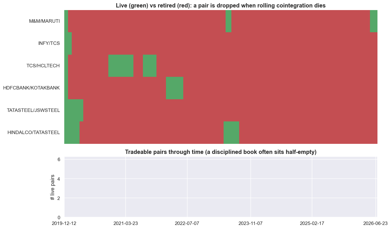
The result is humbling, and it is the truest number in the chapter. Each pair passes the rolling screen only a sliver of the time - TCS / HCLTECH the most at 13%, INFY / TCS the least at 2% - and the median number of pairs passing the screen is 0 of 6. A disciplined book that obeys its own retire rule sits empty more often than not. Put plainly: these relationships are cointegrated occasionally, not reliably. A fixed six-pair book that ignores the screen is mostly running on faith, trading relationships that have already ended, because the entry logic never checked whether the link still held.

Where this breaks

A portfolio layer makes a stat-arb book survivable. It does not make a weak edge strong. And every tool above leans on estimates that are themselves fragile.

• The covariance is estimated, and it moves. Shrinkage cut the 63-day condition number from 6.9 to 2.3 - more stable, not more correct. The shared-leg correlations that drive the weights drift over time, so a weight fitted on 2019-2023 can be wrong out of sample. Shrinkage buys stability, not foresight.
• Neutralisation only looks backward. The leg betas, hedge ratios and the NIFTY overlay are all fitted on past data. The leftover beta we "hedged to zero" is zero only in-sample. Out of sample the book carries beta again, and the high-hedge-ratio M&M / MARUTI pair (beta -1.11) leaks the most, exactly when it hurts.
• Stops and throttles cut both ways. The stop that cost a 21.4% reversion is the same one that caps an unlimited loss on a truly broken pair. No threshold resolves the trade-off. Tuning it on past data just fits it to last time's mistake.
• Retiring lags. A rolling cointegration screen only confirms a break after a 252-day window moves - most of the loss is taken before the rule fires, and re-admission can whipsaw. By that screen, the median tradeable count was 0 of 6.
• Six survivors, weighted with hindsight. This book is built from today's index names that happened to test cointegrated on the train window. That is the same survivorship bias the single-pair teardown measured, now multiplied across six pairs, with the delisted and merged pairs nowhere in sight.

The honest summary: this is research-grade portfolio construction built on a research abstraction. It is the right way to turn signals into a book, and it clearly improves the ride - out-of-sample net Sharpe from 0.34 to 0.43, worst drawdown from -13.8% to -10.0%. But it sits on top of the same thin, cost-heavy, drifting edge. And it carries every caveat of the equity-short problem, which on Indian markets may require stock futures, borrowed stock, or intraday square-off - each one changing costs, margin, borrow availability and risk. A statistical relationship existing is not the same as a tradable edge existing. The portfolio layer is what keeps you in the game long enough to find out which one you have. Educational content only, not investment advice.