Cointegration Mechanics

The last chapter ended with a yes-or-no answer: this pair is cointegrated, that one is not. Cointegration means each stock wanders on its own like a random walk, but a particular combination of the two stays pinned to an average - as if an invisible elastic band ties them together. That yes-or-no answer is actually the least useful thing the test produces. The interesting questions all come after it.

How many units of the second stock do you trade against one unit of the first? That count is the hedge ratio, and we need to know whether it is even well-defined. What does the spread - the combination you actually trade - look like, and how do you prove it gets pulled back to its average instead of just hoping it does? Once it does revert, how long does the return trip take? That waiting time is the half-life, and it doubles as your holding period and your stop-loss horizon. This chapter opens up the Engle-Granger method and walks through every moving part on one real cointegrated NSE pair. We compute each number from the data and, at each step, point out exactly where it is misleading you.

The two-step machine, and a pair the data chooses

Engle-Granger has two steps and nothing more. Step one is an ordinary least squares regression - OLS, the standard line of best fit - of one log price on the other. The slope of that line is the hedge ratio. What the line cannot explain, the leftover, is the spread. Step two checks whether that leftover spread is stationary: does it wander around a fixed average and keep getting pulled back, instead of drifting off forever? If it is stationary, the two prices are cointegrated, and that spread is the thing you trade. Hold this picture in your head, because every code cell below is one box in it.

We do not pick the pair by gut feel. We fix one window of data - 2019-01-01 to 2023-12-29, 1,239 trading days - and hold it for the whole chapter so every number stays comparable. Then we run the Engle-Granger coint test on all ten same-sector pairs among the five Nifty bank names. Holding the window fixed matters. Cointegration is a claim about one particular stretch of data, and quietly changing the window for each pair is one of the easiest ways to fool yourself.

In this window, exactly one of the ten pairs clears the 5% bar: HDFCBANK against KOTAKBANK, with coint p = 0.0306 (t = -3.521 against a 5% MacKinnon critical value of -3.341). The runner-up, HDFCBANK against SBIN, came in at p = 0.096 - on the wrong side of the line. You do not move the threshold after you have seen the number. That single survivor out of ten is your first warning about selection bias, which the next chapter takes on. For now, HDFCBANK is our A and KOTAKBANK is our B. We work in log prices throughout, because a slope measured on logs is a unit-free, return-for-return relationship - exactly what cointegration theory and the half-life assume.

Three hedge ratios, and why OLS lies

The slope from step one is the hedge ratio: how many units of B you trade to cancel one unit of A. The obvious way to get it is sm.OLS(A, B). Here is the trap. OLS assumes the variable on the right-hand side is measured perfectly, with no error, and it only minimises the vertical gaps between the points and the line. But both stocks are noisy. So the answer you get changes depending on which stock you put on the right.

Put A on the left and B on the right, and you get b = 1.0545. Flip it - B on the left, A on the right - and you get b = 0.7859, which translates back into A-on-B terms as 1.2724. If the hedge ratio were a clean physical constant, those two numbers would be exact reciprocals and agree. They do not. They sit on either side of the truth, 20.7% of the OLS value apart. There is an exact reason, and it is worth remembering: the two slopes multiplied together equal the regression R-squared. Here, 1.0545 x 0.7859 = 0.8288 = R-squared. Because R-squared is below one, the two slopes can never be reciprocals, and each one is pulled toward zero. Statisticians call this errors-in-variables, or attenuation, bias. It is not a rounding glitch. It is a 21% disagreement about how big your position should be.

The picture explains when this actually bites. OLS A~B minimises the vertical scatter, which quietly assumes all the noise lives in A and that B is perfectly clean. OLS B~A assumes the reverse. But both legs are noisy stocks, so neither axis is the clean one. The gap between the two slopes depends entirely on R-squared. When R-squared = 1 the two lines sit right on top of each other. As R-squared drops, they fan apart, until the choice of which stock goes on the x-axis dominates the answer. Our tight R-squared of 0.83 makes the 21% gap the mild case. On a noisier pair, the same effect can hand you two hedge ratios that differ by half - and at that point your position is a directional bet wearing a spread's clothing.

On the scatter plot, the three lines look close only because this relationship is genuinely tight (R-squared = 0.83). On a looser pair the fan opens up dramatically. Then your hedge ratio - and therefore your profit and loss - rests on an arbitrary choice of which leg goes on the x-axis.

Copy

# fit the three lines first so we can draw them on the joint scatter
ols_ab = sm.OLS(A, sm.add_constant(B)).fit()                 # A = a + b.B
ols_ba = sm.OLS(B, sm.add_constant(A)).fit()                 # B = c + d.A
b_ab   = ols_ab.params[B_name]
b_ba   = ols_ba.params[A_name]
b_ba_inv = 1.0 / b_ba                                        # express B~A back in A-on-B terms

def _tls_beta(x, y):
    """Total-least-squares slope via orthogonal distance regression (scipy.odr)."""
    f = odr.Model(lambda B_, x_: B_[0] * x_ + B_[1])
    out = odr.ODR(odr.RealData(x.values, y.values), f, beta0=[b_ab, 0.0]).run()
    return out.beta[0], out.beta[1]
b_tls, a_tls = _tls_beta(B, A)

g = sns.jointplot(x=B.values, y=A.values, kind='scatter', height=6.2,
                  s=10, alpha=0.35, color=C['grey'], marginal_kws=dict(bins=40))
xs = np.linspace(B.min(), B.max(), 100)
g.ax_joint.plot(xs, ols_ab.params['const'] + b_ab*xs, color=C['amber'], lw=2.2, label=f'OLS A~B  (b={b_ab:.3f})')
g.ax_joint.plot(xs, (-ols_ba.params['const']/b_ba) + b_ba_inv*xs, color=C['blue'], lw=2.2, label=f'OLS B~A flipped  (b={b_ba_inv:.3f})')
g.ax_joint.plot(xs, a_tls + b_tls*xs, color=C['green'], lw=2.2, ls='--', label=f'TLS orthogonal  (b={b_tls:.3f})')
g.ax_joint.set_xlabel(f'log {B_name}'); g.ax_joint.set_ylabel(f'log {A_name}')
g.ax_joint.legend(fontsize=9, loc='upper left')
g.figure.suptitle(f'{A_name} vs {B_name}: three honest hedge ratios', y=1.02, fontweight='bold')
plt.show()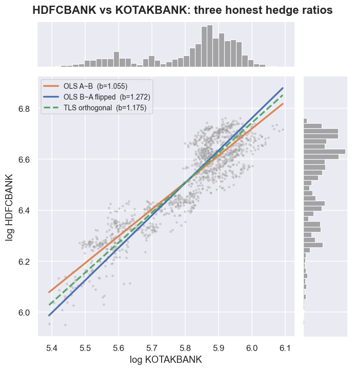

Total least squares: the honest middle line

The fix is to stop pretending either axis is the clean one. Total least squares - also called orthogonal distance regression, available directly as scipy.odr - minimises the perpendicular distance from each point to the line. It treats A and B even-handedly. The answer no longer depends on which series you call x, and it always lands between the two OLS slopes: 1.0545 <= 1.1751 <= 1.2724. The TLS hedge ratio of 1.1751 is 11.4% higher than the OLS A~B value we will actually use.

So which one do we trade on? Engle-Granger is defined on the OLS residual, and with R-squared this high the OLS and TLS spreads behave almost the same. So the rest of this chapter builds the spread from OLS A~B, to match the textbook two-step. TLS is not magic. Its real lesson is simpler: the hedge ratio is an estimate, and it carries an ambiguity about which way you ran the regression. A careful researcher states which convention they used, instead of pretending the number fell from the sky.

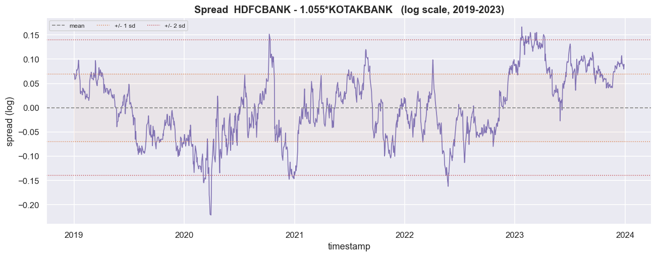
Building the spread, and the formal test that it reverts

With the convention fixed, the spread is simply the leftover from step one: s = A - (alpha + beta.B). Subtracting the fitted beta.B strips out the trend the two banks share - the sector and the wider market. What remains, if the pair is truly cointegrated, swings around a constant level. OLS pins the mean at essentially zero (we measure -0.00000), with a standard deviation of 0.06982 in log units. The series crosses its own mean 59 times in 1,239 days. Crossing often is the visual fingerprint of reversion. A random walk would wander off and cross only rarely.

Copy

alpha, beta = ols_ab.params['const'], b_ab
spread = A - (alpha + beta * B)
spread.name = 'spread'
mu, sd = spread.mean(), spread.std()

fig, ax = plt.subplots(figsize=(12, 4.8))
sns.lineplot(x=spread.index, y=spread.values, color=C['purple'], lw=1.1, ax=ax)
ax.axhline(mu, color=C['grey'], lw=1.2, ls='--', label='mean')
for k, c in [(1, C['amber']), (2, C['red'])]:
    ax.axhline(mu + k*sd, color=c, lw=1.0, ls=':', label=f'+/- {k} sd')
    ax.axhline(mu - k*sd, color=c, lw=1.0, ls=':')
ax.fill_between(spread.index, mu-sd, mu+sd, color=C['amber'], alpha=0.06)
ax.set_title(f'Spread  {A_name} - {beta:.3f}*{B_name}   (log scale, {WIN0[:4]}-{WIN1[:4]})')
ax.set_ylabel('spread (log)'); ax.legend(ncol=5, fontsize=8, loc='upper left')
plt.tight_layout(); plt.show()
print(f'spread mean = {mu:.5f} (OLS forces it to ~0)   sd = {sd:.5f}')
print(f'times it crossed its mean in-window: {(np.sign(spread-mu).diff()!=0).sum()}  '
      f'(a reverting spread crosses often)')

Live output

spread mean = -0.00000 (OLS forces it to ~0)   sd = 0.06982
times it crossed its mean in-window: 59  (a reverting spread crosses often)

A spread that wobbles on a chart is suggestive, not proof. The formal test is the ADF test (Augmented Dickey-Fuller), which asks one question: is this series a random walk, or does it mean-revert? Its p-value is the chance, if the spread really were just a random walk, of seeing a result at least this extreme. Small (below 0.05) is evidence of reversion; large means you cannot rule out a random walk. Here is the subtle point that separates a careful researcher from an optimist. Run adfuller directly on the OLS residual and you get a t-statistic of -3.519 and p = 0.0075 - a strong, confident rejection of the random walk. But that number flatters you. The hedge ratio was fitted on the very data being tested, chosen, in effect, to make the residual look as stationary as possible. The honest number is the Engle-Granger coint p of 0.0306 from the scan, which uses the correct MacKinnon critical values for a hedge ratio that was estimated rather than known. Both clear 5%, so the verdict holds. But notice the gap. The naive ADF p (0.0075) is four times stronger than the honest p (0.0306) on the exact same spread. Always report the conservative one.

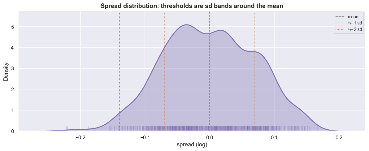
The spread's distribution is roughly bell-shaped and tight - skew -0.02, excess kurtosis -0.52. That shape is what lets us later turn standard-deviation bands into entry and exit thresholds. Near-zero skew means the spread is not lopsided toward one stock. The slightly negative excess kurtosis means thinner tails than a normal bell curve, so the one- and two-standard-deviation bands actually mean what they claim. A later chapter turns those exact lines into a rule: short the spread above the upper band, go long below the lower one. That rule only works on a distribution this symmetric and tight. "Mean-reverting" should be something you can see on a chart - and here you can.

Copy

fig, ax = plt.subplots(figsize=(11, 4.6))
sns.kdeplot(spread.values, fill=True, color=C['purple'], alpha=0.35, lw=2, ax=ax)
sns.rugplot(spread.values, color=C['purple'], alpha=0.25, height=0.04, ax=ax)
ax.axvline(mu, color=C['grey'], ls='--', lw=1.2, label='mean')
for k, c in [(1, C['amber']), (2, C['red'])]:
    ax.axvline(mu + k*sd, color=c, ls=':', lw=1.1)
    ax.axvline(mu - k*sd, color=c, ls=':', lw=1.1, label=f'+/- {k} sd')
from scipy import stats as _st
print(f'skew = {_st.skew(spread):+.2f}   excess kurtosis = {_st.kurtosis(spread):+.2f}  '
      f'(0/0 would be perfectly normal)')
ax.set_title('Spread distribution: thresholds are sd bands around the mean')
ax.set_xlabel('spread (log)'); ax.legend(fontsize=9)
plt.tight_layout(); plt.show()

Live output

skew = -0.02   excess kurtosis = -0.52  (0/0 would be perfectly normal)

How fast it comes home: the OU half-life

Stationarity tells you the spread will come back to its mean. It says nothing about when - and "when" is what you actually trade. To get the timing, model the spread as an Ornstein-Uhlenbeck (OU) process: think of a spring that pulls any deviation back toward the average, harder the further it has strayed. Its discrete, day-by-day version is an AR(1) model, where each step leans back toward the mean. In practice, you regress the daily change ds on yesterday's level s(t-1). The slope is phi, the pull-back speed is kappa = -phi, and the half-life = ln(2) / kappa in trading days. The half-life is how long, on average, a deviation takes to shrink by half - and that is the natural holding period of the trade.

On our spread the AR(1) fit gives phi = -0.0237, so kappa = 0.0237, strongly significant (t = -3.83, p = 0.0001). Read kappa as a decay rate: roughly 2.4% of any gap closes per trading day. Compounded, that means half the gap is gone in ln(2) / 0.0237 = 29.3 trading days - about 1.4 months, just 2.4% of the sample. The significance matters as much as the estimate. A kappa that you cannot tell apart from zero is no reversion at all, just noise that happens to lean the right way. The t of -3.83 is what lets us call this reversion real, rather than an accident of the fit.

Read the half-life as a holding period. A typical deviation is half-gone in roughly six weeks, so you hold a position for days to weeks - not minutes, not years. That one number sets your trade horizon. It also sets your patience: how long you wait before deciding a position is broken rather than just slow. Be wary if the half-life is a large fraction of your sample. That means you have not seen enough complete cycles to trust the reversion is stable, rather than one lucky round trip.

Copy

fig, ax = plt.subplots(figsize=(7.6, 5.6))
sns.regplot(x=h['sl'].values, y=h['ds'].values, ax=ax,
            scatter_kws=dict(s=10, alpha=0.3, color=C['grey']),
            line_kws=dict(color=C['red'], lw=2.4))
ax.axhline(0, color=C['grey'], lw=0.8, ls=':'); ax.axvline(mu, color=C['grey'], lw=0.8, ls=':')
ax.set_xlabel('spread level  s(t-1)'); ax.set_ylabel('next-day change  ds(t)')
ax.set_title(f'AR(1) reversion: slope phi = {h["phi"]:.3f} < 0  =>  half-life {h["half_life"]:.0f}d')
plt.tight_layout(); plt.show()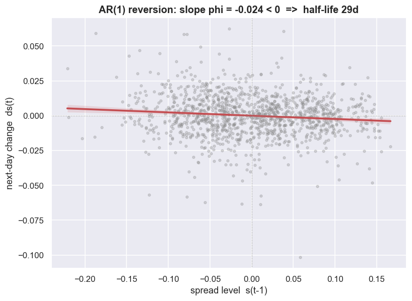

The downward-sloping regression line is the mean reversion, drawn out. When the spread is above its mean, it tends to fall next. When it is below, it tends to rise. A flat line would mean a random walk. An upward-sloping line would mean an explosive series running away from its mean.

The half-life mirage

Here is the trap that catches careful people. The half-life formula always returns a number - even when the spread does not revert at all. A finite, healthy-looking half-life proves nothing on its own. The two gates must be applied in order: first confirm the spread is stationary with the ADF test, then read the half-life. Skip the first gate and the second one lies to you.

To prove it, line up the real spread against three made-up controls of the same length. First, a pure random walk - a series whose next value is just today's value plus random noise, with no home to come back to. It reports kappa = 0.0025 and a half-life of 280 days, but its ADF p is 0.157, so it is not stationary and that half-life means nothing. Second, an explosive series (rho > 1): it gives kappa = -0.0100, a negative number, so its half-life is simply undefined. Third, the dangerous one - a near-unit-root drift. It posts kappa = 0.0108, positive, with a half-life of 64 days that looks perfectly tradeable. But its ADF p is 0.106, so it fails the stationarity gate outright. That 64-day half-life is a mirage. If you had trusted it without testing stationarity first, you would have sized a position into a series that never comes home.

Copy

fig, axes = plt.subplots(2, 2, figsize=(12, 6.4), sharex=True)
for ax, (name, ser) in zip(axes.ravel(), controls.items()):
    z = (np.asarray(ser, float) - np.nanmean(ser)) / np.nanstd(ser)   # standardise to compare shapes
    col = C['green'] if name.endswith('(real)') else C['grey']
    ax.plot(z, color=col, lw=0.9)
    ax.axhline(0, color=C['amber'], lw=1.0, ls='--')
    ax.set_title(name, fontsize=10.5)
    ax.set_ylabel('z')
fig.suptitle('Standardised: a tradeable spread keeps coming home; the controls do not',
             fontweight='bold', y=1.01)
plt.tight_layout(); plt.show()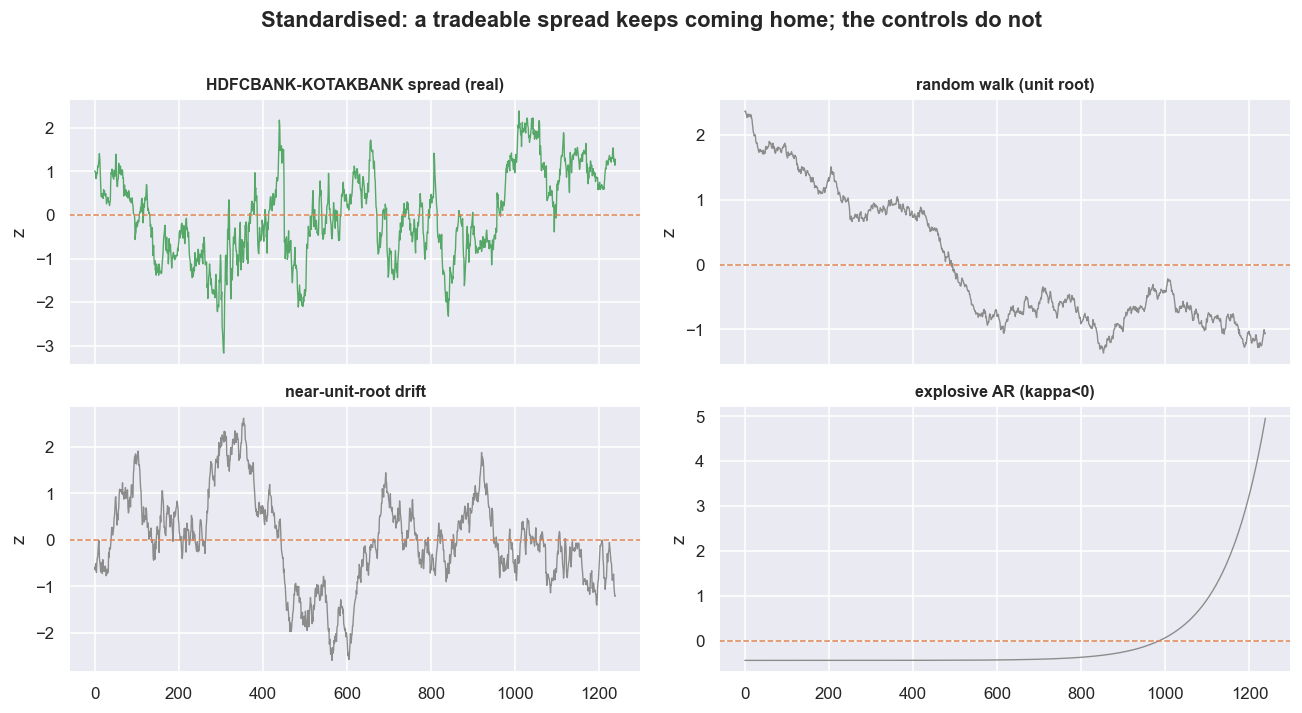

Plotted side by side on the same scale, only the real HDFCBANK-KOTAKBANK spread keeps coming back to its centre. The random walk and the near-unit-root drift wander off and stay gone. The near-unit-root case is the one you meet in the wild: a pair that is almost cointegrated, drifting slowly enough that the half-life reports a believable 64 days while the relationship is quietly broken. The ADF test is the only thing standing between you and that trap - and only if you run it before the half-life tempts you.

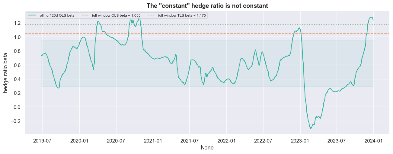
And there is one more crack, even in this genuine pair. We estimated a single beta over the whole window. But a trailing 120-day OLS hedge ratio swings from -0.312 to 1.297 - a range of 258% of its own mean of 0.624. The "constant" hedge ratio is anything but constant. This is the whole reason a later chapter builds a dynamic, Kalman-updated hedge ratio. A fixed-beta spread fitted on the data you built the model with (in-sample) will drift out of its bands on fresh data you never touched (out-of-sample), for reasons that have nothing to do with reversion.

Copy

def rolling_beta(A, B, w=120):
    """Trailing-window OLS slope of A on B, using only data up to each point (no look-ahead)."""
    idx, out = A.index, []
    Av, Bv = A.values, B.values
    for i in range(w, len(A)):
        bb = np.polyfit(Bv[i-w:i], Av[i-w:i], 1)[0]
        out.append((idx[i], bb))
    return pd.Series(dict(out))

rb = rolling_beta(A, B, w=120)
fig, ax = plt.subplots(figsize=(12, 4.8))
sns.lineplot(x=rb.index, y=rb.values, color=C['teal'], lw=1.6, ax=ax, label='rolling 120d OLS beta')
ax.axhline(b_ab,  color=C['amber'], ls='--', lw=1.4, label=f'full-window OLS beta = {b_ab:.3f}')
ax.axhline(b_tls, color=C['green'], ls=':',  lw=1.4, label=f'full-window TLS beta = {b_tls:.3f}')
ax.fill_between(rb.index, rb.mean()-rb.std(), rb.mean()+rb.std(), color=C['teal'], alpha=0.08)
ax.set_title('The "constant" hedge ratio is not constant'); ax.set_ylabel('hedge ratio beta')
ax.legend(fontsize=8, ncol=3, loc='upper left')
plt.tight_layout(); plt.show()
print(f'rolling beta: min {rb.min():.3f}  max {rb.max():.3f}  mean {rb.mean():.3f}  sd {rb.std():.3f}')
print(f'range as a fraction of the mean: {(rb.max()-rb.min())/abs(rb.mean())*100:.0f}%  '
      f'-- a single fixed beta hides a lot of drift')

Live output

rolling beta: min -0.312  max 1.297  mean 0.624  sd 0.331
range as a fraction of the mean: 258%  -- a single fixed beta hides a lot of drift

Check yourself

1. What is the hedge ratio, and what happens if it is wrong or stale?

It is how many units of one stock you hold against one unit of the other so their shared market moves cancel. Get it wrong and the "spread" still carries market direction - your market-neutral trade is secretly a directional bet.

2. Why is the plain ADF p-value on the residual (0.0075) more flattering than the Engle-Granger coint p (0.0306)?

The hedge ratio was fitted on the very data being tested, in effect chosen to make the residual look as stationary as possible. Engle-Granger uses the correct critical values for an estimated ratio, so it is the honest number. Always report the conservative one.

3. A spread has a half-life of 24 days. What does that tell a trader?

How long a deviation takes, on average, to shrink by half - your natural holding period. Short half-lives are forgiving; long ones mean months of financing, borrow and headline risk on two legs while you wait.

Where this breaks

Every box in the Engle-Granger diagram is an assumption that can fail. Here they are, in rough order of how often each one kills a real pair:

• Hedge-ratio instability is the big one. The rolling beta wandered across a range equal to 258% of its mean. Engle-Granger assumes one hedge ratio that holds for all time. When beta drifts, the fixed-beta spread is mis-hedged, leaks directional risk, and breaks through its bands for reasons unrelated to reversion. Rolling-OLS or a Kalman filter can chase the drift, but every extra knob you add is a fresh chance to overfit.
• The x-versus-y ambiguity is real money. OLS A~B gave 1.0545; the flip gave 1.2724 - a 20.7% disagreement on a tight pair. On a looser pair it is far worse, and your profit and loss then hangs on a modelling choice rather than on the market. TLS is more honest, but it still assumes a single, constant ratio.
• In-sample cointegration is an overfit waiting to happen. We scanned ten bank pairs and reported the one that passed at p = 0.0306. That is the best of ten tests dressed up as a single result - classic selection bias. The next chapter puts real numbers on how many fake "cointegrated" pairs pure noise can manufacture once you scan a whole universe.
• The half-life is fragile out-of-sample. The 29.3-day figure is an in-sample estimate with wide error bars. A value that looks tradeable in this window can lengthen, vanish, or even turn negative in the next. A spread whose half-life blows up is a position that simply does not come back. Re-estimate it out-of-sample, every time.
• ADF on a fitted residual flatters you. The naive ADF p (0.0075) was four times stronger than the honest coint p (0.0306) on the identical spread, precisely because the residual had been optimised first. Report the conservative number.
• Stationary in logs is not tradeable in rupees. This whole chapter lives in adjusted log prices. Costs, the bid-ask spread crossed on two legs, the borrow cost on the short, and the gap between adjusted and actually tradable prices are all still ahead of us. Treat the short leg as a research abstraction until you have a real way to implement it. In Indian markets that may mean stock futures, borrowed stock, or intraday square-off - and each choice changes costs, margin, borrow availability, taxes, slippage and risk. A statistical relationship existing is not the same as a tradable edge existing.

The next chapter takes on the selection-bias problem this one walked into on purpose: how to scan a whole universe for cointegrated pairs without manufacturing false discoveries out of pure noise.