Capstone: The Honest Stat-Arb Workflow

Sixteen chapters ago we made one promise: to draw a single bright line between a statistical relationship and a tradable edge, and to never let a pretty number talk us across it. Everything since has been the machinery for holding that line. Cointegration tests. Spread construction. Signal design. Cost models. Out-of-sample discipline - always judging a model on fresh data it never saw while it was built. And a long parade of techniques that looked brilliant on the data they were tuned on and humbling on data they had not seen. This final chapter teaches no new trick. It assembles every earlier piece into one disciplined workflow you can run start to finish, then reads back the honest scorecard of what actually survived. The course has been deliberately brutal because the subject is. What is left at the end is small, hard-won, and real - and knowing exactly how small is the whole point.

One chain, six links

A stat-arb programme is not a single strategy. It is a chain of steps, and every link can quietly break the one after it. Get the universe wrong, and your cointegration test is just mining noise. Trust correlation instead of cointegration, and you pick pairs with nothing holding them together. Freeze a hedge ratio, and the spread mis-hedges the moment the market regime turns. The workflow below is the same chain the companion notebooks walk, in order, and no step can be skipped.

What each link actually taught

Data and universe come first, because every statistic downstream inherits their flaws. We limited the search to liquid, F&O-eligible stocks in the same sector - which gives them an economic reason to move together - and used historical adjusted closes from our research universe (corrected for splits and dividends), with the survivorship limits already acknowledged. That is not the same as a full point-in-time institutional database. The closing price is the right price to learn from: one clean, comparable, auction-settled number per stock per day, exactly what a cointegration test wants. But it is the wrong price to trade at: you cannot transact at an adjusted close, and your real fill lands on the next bar. Holding both ideas at once is the discipline the whole course is built on.

Cointegration, not correlation, is the entry exam. These two sound similar but are not. Correlation measures whether two stocks move together day to day. Cointegration is a stronger, longer-run idea: each price wanders on its own, but a particular combination of them stays tied together, as if by an invisible elastic band. Across 75 same-sector pairs, the rank correlation between return-correlation and the cointegration p-value - where a small value is good evidence the pair is genuinely tied - was -0.04, statistically indistinguishable from zero. The most correlated pair in the table drifted apart and never came back. Weaker-correlated pairs reverted cleanly. Screen on the wrong one and you keep picking spreads with no centre of gravity.

Finding pairs without fooling yourself is mostly a defence against your own search. Run a cointegration test over hundreds of pairs and a handful will pass at 5% by pure luck. It is the same trap that makes 90% of unrelated random walks - prices that are just today's value plus noise, with no home to return to - look "significant" when you compare their levels. The honest screen starts from an economic reason to pair two stocks, controls the false-discovery rate (the share of your "winners" that are flukes), and treats any low p-value pulled from a big scan as a hypothesis, never a discovery.

Spread and signal is the only step that is genuinely mechanical. You estimate a cointegrating hedge ratio - how many units of one stock to trade against the other so their shared market moves cancel - rather than using the raw price ratio, which silently assumes that ratio is one. You build a trailing rolling z-score - how many standard deviations the spread sits from its own recent average - sized to the spread's own half-life, the time a deviation takes to shrink by half. Then a four-zone rule: enter in a band, exit at the average, hard-stop beyond it, always filled on the next bar, never the same one. Built cleanly, this prints a gorgeous curve on the data it was tuned on. On HDFCBANK against KOTAKBANK: +98% gross at a 0.99 Sharpe, a 72% hit rate, and zero stops triggered. Every number true - in that window, in-sample, and gross, meaning before trading costs. None of it a forecast.

The honest scorecard

Then comes link five, where most ideas die and where the course earns its keep. We took every tempting in-sample result out of sample, subtracted realistic NSE costs on two legs traded twice, and asked whether the relationship was even stable. Here is the whole arc on one page.

Technique	Headline (in-sample / gross)	Honest verdict (net, out-of-sample)
Naive pairs (HDFCBANK / KOTAKBANK)	net Sharpe 1.01	net Sharpe 0.34 - two-thirds gone
Dynamic hedge (Kalman beta)	promised adaptivity	OOS net -1.50 vs static +0.76; 0 of 20 grid settings beat the static beta
Basket (Johansen, 5 banks)	94% of sub-baskets stationary	0% still stationary out-of-sample
Cross-sectional factor-neutral	gross Sharpe 1.34	net Sharpe -1.99 under turnover
Portfolio of 6 vol-targeted pairs	net Sharpe 0.94	net Sharpe 0.43 out-of-sample

Read that table slowly, because it is the course. The naive pair was not a bug. It was a clean, correct build whose edge was mostly a feature of the window it was tuned on. Held blind, it kept barely a third of its Sharpe, and the pair failed the cointegration test in about 90% of rolling windows. The Kalman filter - a method that nudges the hedge ratio a little each day as new prices arrive, instead of fixing it once - was the "obvious" fix for a drifting hedge ratio. It did not just underperform the frozen beta. It lost money out of sample, and no setting on a 20-point grid beat the static bar, because a hedge ratio that chases noise mis-hedges more than a stale one does. The Johansen basket - the multi-stock version of a cointegration test, which hunts for a stationary combination of several stocks at once - was the sharpest trap. 94% of candidate baskets tested stationary in-sample, and exactly none survived, because a k-leg basket has k-1 free weights to estimate, and estimation error is where baskets go to die.

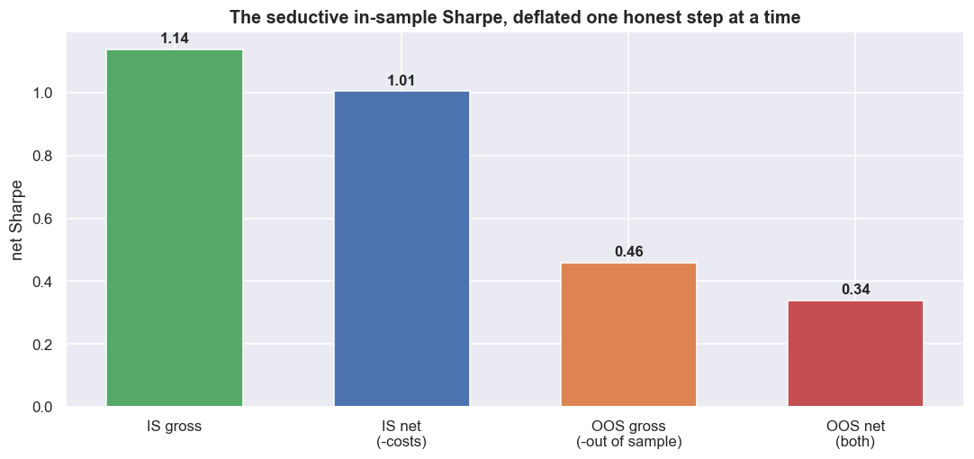
The flagship pair makes that deflation concrete. Every honest step, taken in order, knocks the tempting number down toward zero. Nothing here is a leak. It is the same strategy seen through progressively less flattering glass.

Copy

# pull together every number into one honest scorecard
def row(label, ret, sl):
    p = perf(ret.loc[sl])
    return dict(view=label, Sharpe=round(p['sharpe'],2), ann_vol=round(p['vol']*100,1),
                total_pct=round(p['total']*100,1), maxDD_pct=round(p['maxdd']*100,1))

card = pd.DataFrame([
    row('IN-SAMPLE  gross',      bt['gross'], isS),
    row('IN-SAMPLE  net',        bt['net'],   isS),
    row('OUT-OF-SAMPLE  gross',  bt['gross'], ooS),
    row('OUT-OF-SAMPLE  net',    bt['net'],   ooS),
    dict(view='WALK-FORWARD 2024+ net', Sharpe=round(perf(wf.loc["2024-01-01":])['sharpe'],2),
         ann_vol=round(perf(wf.loc["2024-01-01":])['vol']*100,1),
         total_pct=round(perf(wf.loc["2024-01-01":])['total']*100,1),
         maxDD_pct=round(perf(wf.loc["2024-01-01":])['maxdd']*100,1)),
]).set_index('view')
print(card.to_string())

# the Sharpe waterfall: where the seductive in-sample number goes
stages = ['IS gross', 'IS net\n(-costs)', 'OOS gross\n(-out of sample)', 'OOS net\n(both)']
vals   = [perf(bt['gross'].loc[isS])['sharpe'], perf(bt['net'].loc[isS])['sharpe'],
          perf(bt['gross'].loc[ooS])['sharpe'], perf(bt['net'].loc[ooS])['sharpe']]
fig, ax = plt.subplots(figsize=(10, 4.8))
cols = [C['green'], C['blue'], C['amber'], C['red']]
bars = ax.bar(stages, vals, color=cols, width=0.6)
for bbar, v in zip(bars, vals):
    ax.text(bbar.get_x()+bbar.get_width()/2, v+0.02, f'{v:.2f}', ha='center', fontsize=11, fontweight='bold')
ax.axhline(0, color=C['grey'], lw=1.0)
ax.set_ylabel('net Sharpe'); ax.set_title('The seductive in-sample Sharpe, deflated one honest step at a time')
plt.tight_layout(); plt.show()

Live output

Sharpe  ann_vol  total_pct  maxDD_pct
view                                                         
IN-SAMPLE  gross          1.14     16.4      134.2      -20.5
IN-SAMPLE  net            1.01     16.4      110.5      -20.9
OUT-OF-SAMPLE  gross      0.46     17.8       17.5      -13.8
OUT-OF-SAMPLE  net        0.34     17.8       11.5      -13.8
WALK-FORWARD 2024+ net    0.62     15.1       22.3      -13.3

The cross-sectional book is the most instructive failure of all, because its signal was real.

This is the funnel that every notebook from chapter three onward is really one layer of. Thousands of pairs co-move. Fewer are cointegrated on the data you tested. Fewer still stay cointegrated out-of-sample. Fewer again survive realistic costs. And only what is left at the very bottom is implementable and net-positive.

What would make a model genuinely tradable

The scorecard is not a counsel of despair. It is a specification. A model that clears every bar above is rare, but it is not mythical, and the four things that separate it from a backtest artefact are concrete.

A real short-leg vehicle. Every backtest in this course shorted freely, and that is the single biggest shortcut it took. In Indian cash equities an intraday short is force-closed near the day's end, so you cannot hold an overnight reversion that way. The realistic default is the stock future - liquid in large names and naturally short-able - but it drags in basis, a monthly roll cost, lot-size rounding, margin on each leg, and the Market-Wide Position Limit: cross 95% of it and the name enters a ban period where you cannot add, often exactly when the spread is most crowded. SLB borrow is the cleanest economic match but is thin, lumpy, and can be recalled. No short, no market-neutral trade. And every rule here moves over time - short-leg availability, the F&O ban, the Market-Wide Position Limit, charges, STT, SLB terms and broker margins all change - so verify the latest NSE, SEBI and broker rules before you deploy, and read the numbers in this course as illustrations of the mechanics, not current quotes.

Costs modelled net, on two legs, both ways. A pair round trip is eight fills, each paying statutory charges plus half the spread plus impact. The honest number ranges from tens of basis points for a delivery hold to over 120 bps once you model real effective spreads and impact on two legs intraday. The edge must clear all of it before a single rupee is yours. And the cross-sectional book proves that a real gross signal can sit entirely below that line.

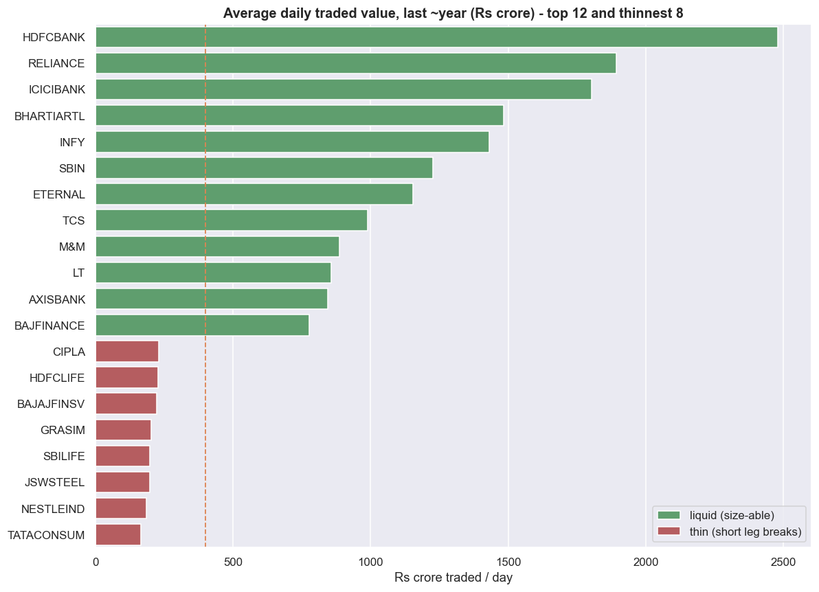
Capacity you can actually fill. A signal that needs more size than the thinner leg can absorb is a paper edge. Liquidity is the first filter, not an afterthought. The range across even a blue-chip universe is wide, and a pair that ties a liquid name to a thin one inherits the thin one's execution problems on both legs.

Copy

# Average daily traded value (ADV) over the last ~year, in Rs crore/day.
adv = {}
for s in UNIVERSE:
    try:
        d = load(s)
        adv[s] = (d['close'] * d['volume']).last('365D').mean() / 1e7
    except Exception as e:
        print('skip', s, e)
adv = pd.Series(adv).sort_values(ascending=False)
show = pd.concat([adv.head(12), adv.tail(8)])
sd = show.reset_index(); sd.columns = ['symbol', 'adv']
sd['tier'] = np.where(sd['adv'] >= adv.median(), 'liquid (size-able)', 'thin (short leg breaks)')
fig, ax = plt.subplots(figsize=(11, 8))
sns.barplot(data=sd, x='adv', y='symbol', hue='tier',
            palette={'liquid (size-able)': C['green'], 'thin (short leg breaks)': C['red']},
            dodge=False, ax=ax)
ax.axvline(adv.median(), color=C['amber'], ls='--', lw=1.2)
ax.set_title('Average daily traded value, last ~year (Rs crore) - top 12 and thinnest 8')
ax.set_xlabel('Rs crore traded / day'); ax.set_ylabel(''); ax.legend(loc='lower right')
plt.tight_layout(); plt.show()
print(f'liquidity span in this window: richest {adv.index[0]} ~Rs {adv.iloc[0]:,.0f} cr/day  '
      f'vs thinnest {adv.index[-1]} ~Rs {adv.iloc[-1]:,.0f} cr/day  ->  '
      f'{adv.iloc[0]/adv.iloc[-1]:.0f}x apart')
print(f'median name trades ~Rs {adv.median():,.0f} cr/day; '
      f'{(adv < adv.median()/3).sum()} names trade under a third of the median.')

Live output

liquidity span in this window: richest HDFCBANK ~Rs 2,479 cr/day  vs thinnest TATACONSUM ~Rs 164 cr/day  ->  15x apart
median name trades ~Rs 399 cr/day; 0 names trade under a third of the median.

Validation that does not flatter. Naive cross-validation leaks through overlapping labels (Sharpe 0.78). Purged-and-embargoed cross-validation, which removes that leak, cut it to 0.50. Now adjust the best-of-many-trials Sharpe for the search itself, and the Deflated Sharpe sits at 0.96 with a 54% probability of backtest overfitting (PBO) - the chance your best-looking setting is just luck that won't repeat. That is barely better than a coin flip that the search found anything real. The out-of-sample Sharpe of 0.34 carries a 95% bootstrap interval of [-0.47, 1.15] that comfortably contains zero, with a 20% probability the true Sharpe is negative. A single backtested number, with no uncertainty shown beside it, is the optimistic end of a range, not the answer.

The pre-trade checklist

Before a single rupee of real capital touches a stat-arb idea, it must pass nine gates. A NO on any one of them does not mean trade smaller. It means the idea goes back to research, not to the order book.

Run the engine yourself

None of this is meant to be taken on faith. The entire research engine is open for you to run, break, and modify. The companion Jupyter notebooks in the Statistical Arbitrage folder of the OpenAlgo Tutorials repository are self-contained and reproduce every number in this course on real NSE closes. 00b is the research-to-real bridge and this checklist. 02 through 06 build stationarity, cointegration, pair-finding, and the signal. 07 is the brutal reality check. 08 is the Kalman that lost. 09 the Johansen baskets. 10 the cross-sectional book that inverted. 11 risk and portfolio construction. 12 the honest validation. And 13 the implementation pathways. Change the pair, change the window, change the cost assumption, and watch the verdict move. That movement is the lesson: a result that flips when you nudge a window was never a result.

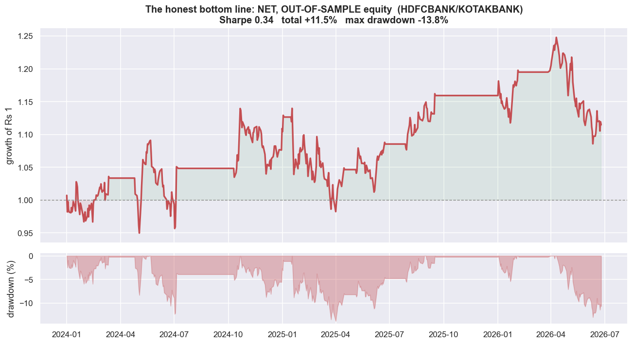
Strip away every flattering layer and one curve is left: the flagship pair, net of realistic costs, out of sample, with every drawdown intact. It is the only line that matches money you could actually have kept. It is the one an honest researcher leads with, not the one a brochure crops out.

Copy

# The chart you are not allowed to hide: the honest, net, out-of-sample equity curve.
no  = eqc(bt['net'].loc[ooS]); p = perf(bt['net'].loc[ooS])
dd  = no/no.cummax() - 1
fig, (ax1, ax2) = plt.subplots(2, 1, figsize=(12, 6.6), sharex=True,
                               gridspec_kw=dict(height_ratios=[3, 1]))
ax1.plot(no.index, no.values, color=C['red'], lw=2.2)
ax1.axhline(1, color=C['grey'], lw=1.0, ls='--')
ax1.fill_between(no.index, 1, no.values, where=(no.values>=1), color=C['green'], alpha=0.10)
ax1.fill_between(no.index, 1, no.values, where=(no.values< 1), color=C['red'],   alpha=0.10)
ax1.set_ylabel('growth of Rs 1')
ax1.set_title(f'The honest bottom line: NET, OUT-OF-SAMPLE equity  ({A_name}/{B_name})\n'
              f'Sharpe {p["sharpe"]:.2f}   total {p["total"]*100:+.1f}%   max drawdown {p["maxdd"]*100:.1f}%')
ax2.fill_between(dd.index, dd.values*100, 0, color=C['red'], alpha=0.35)
ax2.set_ylabel('drawdown (%)'); ax2.set_xlabel('')
plt.tight_layout(); plt.show()

print(f'Net of realistic NSE costs, out of sample, over {(pd.Timestamp(OO1)-pd.Timestamp(OO0)).days/365.25:.1f} years,')
print(f'this much-celebrated pair returned {p["total"]*100:+.1f}% at a Sharpe of {p["sharpe"]:.2f} -- before a single')
print(f'rupee of borrow cost, financing, slippage beyond our estimate, or the equity-short problem. That is the truth.')

Live output

Net of realistic NSE costs, out of sample, over 2.5 years,
this much-celebrated pair returned +11.5% at a Sharpe of 0.34 -- before a single
rupee of borrow cost, financing, slippage beyond our estimate, or the equity-short problem. That is the truth.

Where this breaks

Even this summary is provisional, and the honest caveats are the same ones that have shadowed every chapter.

• Every number is specific to this window. Different universes, windows, and cost models give different verdicts. The scorecard is a faithful account of one decade of NSE data, not a law of markets. Re-run it on yours.
• The short leg is still assumed. The whole course shorts freely on equity closes. Real implementation needs a futures, SLB, or intraday vehicle, each with basis, roll, borrow, margin, and ban risk the backtests never paid for.
• Survivorship flatters all of it. The universe is today's index members looking back. The pairs that merged or delisted never entered the search, so even the humbling numbers are the flattering version.
• The survivor is marginal, not safe. The risk-managed book's out-of-sample Sharpe near 0.43 is the best honest result in the course, and it is still thin, cost-sensitive, borrow-dependent, and one regime shift from breaking. A small allocation, watched closely, with a kill switch - not a livelihood.
• Crowding makes the edge a shared one. Thousands of desks run the same screens. Being market-neutral to the index is not the same as being neutral to other arbitrageurs deleveraging into you.

If you take one sentence from seventeen chapters, take the one the whole course was built to earn: a statistical relationship is not a tradable edge. Educational content only, not investment advice.

Glossary: the terms in one place

Every term the course uses, in one plain-English list to flip back to.

• ADF test (Augmented Dickey-Fuller) - asks whether a series is a random walk or mean-reverts. A small p-value is evidence of mean reversion.
• AR(1) / OU process - simple models of a mean-reverting series, where each step leans back toward the average.
• Basis - the gap between a future's price and the underlying spot price; it moves and must be carried and rolled.
• Beta (market) - how much a stock moves for a one-unit move in the market; used to size a hedge.
• Bonferroni / Benjamini-Hochberg - corrections that tighten the p-value threshold when you run many tests, to control false positives.
• Cointegration - each price wanders like a random walk, but a particular combination of them is stationary, as if tied by an invisible elastic band.
• Cointegrating vector - the set of basket weights that Johansen finds to be stationary; your portfolio weights.
• Confidence interval - a range that, with stated confidence (say 95%), is built to capture the true value most of the time. Wide means you know little.
• Deflated Sharpe - a Sharpe ratio discounted for how many strategies you tried, so luck does not masquerade as skill.
• Dollar-neutral vs beta-neutral - dollar-neutral is equal money long and short; beta-neutral is sized so market moves cancel. Not the same thing.
• Engle-Granger - the two-step cointegration test for a pair: fit the hedge ratio, then test the residual for stationarity.
• Gross vs net - gross is before trading costs, net is after. Stat arb lives or dies on net.
• Half-life - how long a deviation takes, on average, to shrink by half; in practice, the natural holding period.
• Hedge ratio - how many units of one stock you trade against one unit of another so their shared market moves cancel.
• Hurst exponent - a position on a line: near 0.5 is a random walk, below 0.5 mean-reverting, above 0.5 trending. One clue, not a proof.
• I(0) / I(1) - I(0) is already stationary (a return); I(1) needs differencing once to become stationary (a price).
• In-sample vs out-of-sample - in-sample is the data you fit on; out-of-sample is fresh data you never touched, the only honest test.
• Johansen test - finds stationary combinations among several stocks at once; the multi-stock version of cointegration.
• Kalman filter - nudges the hedge ratio a little each day as new prices arrive, instead of fixing it once.
• KPSS test - the mirror of ADF: its null is stationary, so it is run alongside ADF for a second opinion.
• Look-ahead bias - using information in a backtest that you could not have known at the time; it manufactures fake edge.
• Market impact / slippage - the price moves against you as you trade; bigger orders pay more. A real cost the close price hides.
• MWPL / F&O ban - the Market-Wide Position Limit; cross it and a name enters a ban period where you cannot add.
• Multiple testing - run enough tests and some pass by luck. Searching a universe for pairs is the classic trap.
• Null vs alternative hypothesis - the boring default a test tries to reject (null) versus the claim you need evidence for (alternative).
• OLS - ordinary least squares, the standard line-of-best-fit regression, used here to estimate the hedge ratio.
• PBO (probability of backtest overfitting) - the chance your best-looking backtest setting is just luck that will not repeat.
• P-value - the chance, if the null were true, of a result at least this extreme. Not the probability the null is true.
• Random walk - a price whose next value is today's plus random noise, with no home value to return to.
• Sharpe ratio - return divided by risk (volatility). Higher is better; below about 1 after costs is weak.
• SLB (securities lending and borrowing) - the regulated way to borrow stock to short it; the cleanest short, but thin and recallable.
• Spread - what is left after you subtract one stock (scaled by the hedge ratio) from another; the thing a pairs trade bets on.
• Spurious regression - a confident but fake relationship that OLS reports between two unrelated trending series.
• Standard error - the standard deviation of an estimate; it shrinks as the sample grows. Small samples give jumpy estimates.
• Stationary / mean-reverting - a series that wanders around a fixed average and keeps getting pulled back; the opposite of a random walk.
• Survivorship bias - studying only today's survivors flatters every backtest, because the names that died never enter the search.
• Turnover - how much of the book you trade over a period; high turnover means costs pile up fast.
• Type I / Type II error - a false positive (finding a pair that is not there) versus a false negative (missing a real one).
• Walk-forward / purged CV - validation that always tests on data after the fit, with gaps to stop information leaking across the boundary.
• Z-score - how many standard deviations the spread sits from its own average right now; the entry and exit gauge.