Honest Backtesting and Validation
The full validation scorecard: walk-forward, purged and embargoed cross-validation, the deflated Sharpe, the probability of backtest overfitting, a blocked bootstrap, and parameter-stability maps.
- ·Walk-forward distributions
- ·Why ordinary CV leaks
- ·Purged and embargoed CV
- ·The deflated Sharpe
- ·Probability of backtest overfitting
- ·Ridge vs plateau
A backtest is a measurement, and the act of searching quietly contaminates it. A backtest simply replays a trading rule over past data to see how it would have done. Every threshold you tried, every window you swept, every pair you scanned uses up a little of your statistical confidence. By the time a strategy "works", you have often just tested it into existence. The previous chapters took the HDFCBANK / KOTAKBANK pairs trade out of sample once and watched the tempting in-sample net Sharpe of 1.01 collapse to 0.34. (In-sample is the data you used to build and tune the rule; out-of-sample is fresh data you never touched - the only honest test. The Sharpe ratio is return divided by risk.) That was the first line of defence. This chapter is the full validation scorecard - the battery of tests a quant runs before believing a single number, run on the same pair and the same z-score rule, with the real numbers in this data window. The point is not to bless the backtest. It is to subtract the part that was never real and report what little is left, without flinching.
The validation funnel: each ring subtracts edge that was never real
A single backtest answers exactly one question - could a rule have fit this past? - and the answer is almost always yes. Validation is a funnel that asks the harder questions one after another, and each question removes some apparent edge. What drips out of the bottom is the honest part. Keep this picture in mind for the whole chapter. The wide mouth is the tempting in-sample Sharpe. Every ring below it is one section that follows.
The setup on trial is the same as before. The spread is s = A - b.B in log prices. The hedge ratio b is estimated on the 2019-2023 train window and then frozen. We use a trailing 60-day z-score, enter at plus-or-minus two, exit at the mean, hard-stop at four, fill on the next bar, and charge realistic delivery (CNC) costs on every position change. Every test below works on the one daily net-return series this produces. Keep two reference numbers in mind throughout: in-sample net Sharpe near 1.0, out-of-sample near 0.3.
Walk-forward: the distribution, not the average
One out-of-sample number is just a single draw from a noisy process. Quote it on its own and you are bluffing. Walk-forward testing turns that one held-out test into many. You estimate the hedge ratio on data up to a cut-off date, trade the next block blind, step the cut-off forward, and repeat. Each block is called a fold. The anchored version grows the training window from a fixed start. The rolling version uses a fixed-length trailing window that forgets old regimes. The honest output is never the average. It is the whole spread of fold Sharpes.
idx = px.index
def make_folds(test_len=126, min_train=504):
    folds, start = [], min_train
    while start + test_len <= len(idx):
        folds.append((start, min(start + test_len, len(idx)))); start += test_len
    return folds
FOLDS = make_folds()

def wf_fold_sharpes(mode, lookback=504):
    out = []
    for ts, te in FOLDS:
        tr = slice(idx[0], idx[ts-1]) if mode == 'anchored' else slice(idx[max(0, ts-lookback)], idx[ts-1])
        bb = fit_beta(tr)
        net = daily_net(bb)
        out.append(dict(fold_start=idx[ts].date(), sharpe=sharpe(net.loc[idx[ts]:idx[te-1]])))
    return pd.DataFrame(out)

wfa = wf_fold_sharpes('anchored'); wfr = wf_fold_sharpes('rolling')
tidy = pd.concat([wfa.assign(scheme='anchored'), wfr.assign(scheme='rolling')], ignore_index=True).dropna(subset=['sharpe'])

fig, (axL, axR) = plt.subplots(1, 2, figsize=(13, 5.0), gridspec_kw=dict(width_ratios=[2, 3]))
sns.boxplot(data=tidy, x='scheme', y='sharpe', hue='scheme', palette=[C['blue'], C['teal']], width=0.5, ax=axL, legend=False)
sns.stripplot(data=tidy, x='scheme', y='sharpe', color='white', edgecolor=C['grey'], linewidth=0.6, size=6, ax=axL)
axL.axhline(0, color=C['red'], ls='--', lw=1.2)
axL.axhline(sharpe(r_is), color=C['green'], ls=':', lw=1.4)
axL.text(1.5, sharpe(r_is), ' in-sample', color=C['green'], fontsize=9, va='center')
axL.set_title('Distribution of OOS fold Sharpe'); axL.set_ylabel('annualised Sharpe (per fold)'); axL.set_xlabel('')

axR.axhline(0, color=C['red'], ls='--', lw=1.1)
axR.plot(wfa['fold_start'], wfa['sharpe'], 'o-', color=C['blue'], lw=1.4, ms=5, label='anchored')
axR.plot(wfr['fold_start'], wfr['sharpe'], 's-', color=C['teal'], lw=1.4, ms=5, label='rolling')
axR.axvspan(pd.Timestamp(OO0), pd.Timestamp(OO1), color=C['amber'], alpha=0.08, label='2024+ (true recent OOS)')
axR.set_title('OOS Sharpe per walk-forward fold, through time'); axR.set_ylabel('fold Sharpe'); axR.set_xlabel('')
axR.legend(fontsize=9, loc='upper right'); axR.tick_params(axis='x', rotation=30)
plt.tight_layout(); plt.show()

for nm, df in [('anchored', wfa.dropna()), ('rolling', wfr.dropna())]:
    s = df['sharpe']
    print(f'{nm:8s}: folds {len(s):2d}   median {s.median():+.2f}   IQR [{s.quantile(.25):+.2f}, {s.quantile(.75):+.2f}]   '
          f'frac>0 {(s>0).mean():.0%}   worst {s.min():+.2f}   best {s.max():+.2f}')
wf_anchored_med = wfa['sharpe'].median(); wf_rolling_med = wfr['sharpe'].median()
wf_frac_pos = (tidy['sharpe'] > 0).mean()
print(f'the in-sample {sharpe(r_is):.2f} sits ABOVE almost every fold: a single backtest reports the best case, not the typical one.')anchored: folds 14 median +0.47 IQR [+0.29, +1.10] frac>0 93% worst -0.96 best +3.30 rolling : folds 14 median +0.57 IQR [+0.10, +1.67] frac>0 86% worst -0.95 best +3.07 the in-sample 1.01 sits ABOVE almost every fold: a single backtest reports the best case, not the typical one.
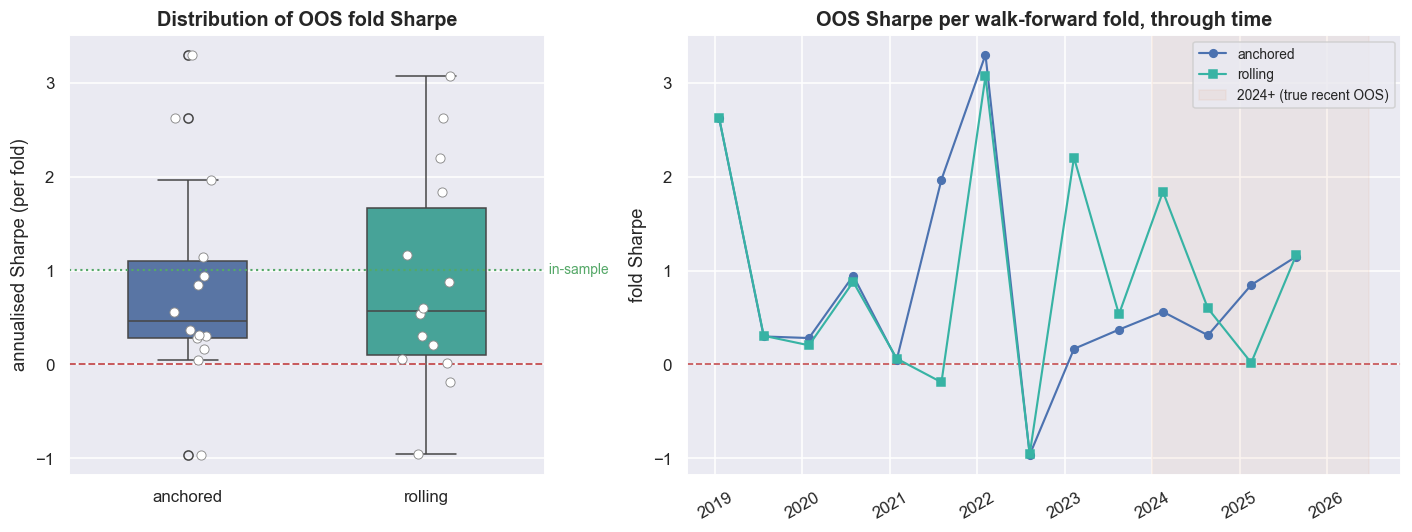
Across 14 folds, the anchored scheme lands a median fold Sharpe of +0.47, with a middle-half range (the interquartile range, where half the folds land) of [+0.29, +1.10]. 93% of folds are positive, but the worst is -0.96 and the best a lucky +3.30. The rolling scheme does slightly better in the middle (median +0.57) and much wider at the extremes (IQR [+0.10, +1.67], worst -0.95). The shape is the tell. This is not a tight cloud sitting confidently above zero. It is a low pile of mediocre folds, with a couple of lucky spikes pulling the average up. And the headline in-sample 1.01 sits above almost every single fold. A lone backtest shows you the best case, not the typical one.
A single out-of-sample Sharpe is one sample from a wide spread of outcomes. When the median fold is roughly half the headline, a quarter of folds are near-flat, and the worst loses money outright, the honest summary is "around 0.5, but I have seen -0.96", not "0.57". Anyone who shows you one number has chosen which draw to show you.
Purged and embargoed cross-validation: ordinary k-fold leaks
The natural next thought is cross-validation. Instead of one cut between train and test, you split the data into many folds and rotate which fold is the test set, then average the results. But ordinary k-fold cross-validation leaks on a trading strategy. The leak is built in, not a bug you can patch. A leak means the test set is secretly contaminated by information from the training set. Two threads tie nearby days together. First, overlapping labels: a reversion trade opened on day t is judged by the spread's move over the next H days, so day t's outcome is built from the same returns as t+1, t+2, and so on - here the holding period is about H = 39 days. Second, trailing features: today's z-score is computed from the prior 60 days. Now shuffle the days into folds at random - the default in almost every library - and nearly every test day has a near-twin sitting in the training set. The model is then tested on data it has effectively already seen.
Measured exactly on this strategy, the fraction of test days that have a training neighbour inside the label window is 100% for shuffled k-fold, 16.6% for blocked (contiguous) folds, and 0% once you purge plus-or-minus H days and add a small embargo. Purging means deleting the training days whose label window overlaps the test block; an embargo adds a short gap after the test block to break any leftover spillover. That leak is not cosmetic - it inflates the score. Pick the entry threshold on each training fold and score it out of fold: the naive shuffled-CV Sharpe is 0.78. Switch to purged and embargoed folds and it drops to 0.50 - a 55% inflation removed. The longer the holding period, the bigger that gap.
# ---- naive (shuffled) vs purged+embargo CV Sharpe, on the OVERLAPPING reversion label -------
cs = np.cumsum(rpair.fillna(0).values); n = len(cs)
fwd = np.full(n, np.nan)
for i in range(n):
    if i + H < n: fwd[i] = cs[i+H] - cs[i]                 # forward H-day spread return
bet = -np.sign(z0.values)                                  # reversion bet direction
outcome = bet * fwd                                        # overlapping H-day outcome
valid = ~np.isnan(z0.values) & ~np.isnan(fwd)
ivd = np.where(valid)[0]
Zv, OUT, POS = np.abs(z0.values[ivd]), outcome[ivd], ivd
m, TAUS = len(ivd), [0.5, 1.0, 1.5, 2.0, 2.5]

def cv_score(IS, OO):
    """Select the entry threshold on IS (max IS reversion-Sharpe), score it on OO."""
    best, bt = -9, TAUS[0]
    for t in TAUS:
        mt = Zv[IS] > t
        if mt.sum() < 40: continue
        o = OUT[IS][mt]; sc = o.mean()/o.std() if o.std() > 0 else -9
        if sc > best: best, bt = sc, t
    mo = Zv[OO] > bt
    if mo.sum() < 20: return np.nan
    o = OUT[OO][mo]
    return o.mean()/o.std()*np.sqrt(ANN/H) if o.std() > 0 else np.nan

rng2 = np.random.default_rng(3)
def cv_shuffled(k=6, reps=60):
    out = []
    for _ in range(reps):
        lab = rng2.integers(0, k, m)
        for f in range(k):
            out.append(cv_score(np.where(lab != f)[0], np.where(lab == f)[0]))
    return np.array(out)
def cv_blocked(k=6, purge=0, emb=0, reps=60):
    out = []
    for _ in range(reps):
        off = rng2.integers(0, m); roll = (np.arange(m) + off) % m
        bb = np.linspace(0, m, k+1).astype(int)
        for f in range(k):
            a, b2 = bb[f], bb[f+1]; OO = roll[a:b2]
            lo, h2 = max(0, a-purge), min(m, b2+purge+emb)
            IS = np.r_[roll[0:lo], roll[h2:m]]
            out.append(cv_score(IS, OO))
    return np.array(out)

cv_naive  = cv_shuffled()
cv_block  = cv_blocked(6, 0, 0)
cv_purged = cv_blocked(6, H, EMB)
cv_naive_m, cv_block_m, cv_purged_m = np.nanmean(cv_naive), np.nanmean(cv_block), np.nanmean(cv_purged)

fig, (a1, a2) = plt.subplots(1, 2, figsize=(13, 4.8), gridspec_kw=dict(width_ratios=[2, 3]))
a1.bar(['shuffled\n(naive)', 'blocked', 'purged+\nembargo'], [leak_shuf, leak_block, leak_purg],
       color=[C['red'], C['amber'], C['green']])
a1.set_ylabel('leak fraction of test days'); a1.set_title('How much each scheme leaks'); a1.set_ylim(0, 1)
for i, v in enumerate([leak_shuf, leak_block, leak_purg]): a1.text(i, v+0.02, f'{v:.0%}', ha='center', fontweight='bold')

bars = a2.bar(['shuffled (naive)', 'blocked', 'purged+embargo'], [cv_naive_m, cv_block_m, cv_purged_m],
              color=[C['red'], C['amber'], C['green']])
a2.axhline(0, color=C['grey'], lw=1.0)
for bbar, v in zip(bars, [cv_naive_m, cv_block_m, cv_purged_m]):
    a2.text(bbar.get_x()+bbar.get_width()/2, v+0.02, f'{v:.2f}', ha='center', fontweight='bold')
a2.set_ylabel('cross-validated Sharpe'); a2.set_title('Naive CV inflates the Sharpe vs purged CV')
plt.tight_layout(); plt.show()

print(f'naive shuffled-CV Sharpe  {cv_naive_m:.2f}   ->   purged+embargo CV Sharpe  {cv_purged_m:.2f}   '
      f'({(cv_naive_m-cv_purged_m)/abs(cv_purged_m)*100:.0f}% inflation removed)')
print(f'the leak enters through the SHUFFLE (near-duplicate neighbours land in both train and test); moving to')
print(f'contiguous blocks and then purging + embargoing the overlap progressively removes it -- and the purge')
print(f'matters more the longer positions are held (here H={H}d).')naive shuffled-CV Sharpe 0.78 -> purged+embargo CV Sharpe 0.50 (55% inflation removed) the leak enters through the SHUFFLE (near-duplicate neighbours land in both train and test); moving to contiguous blocks and then purging + embargoing the overlap progressively removes it -- and the purge matters more the longer positions are held (here H=39d).
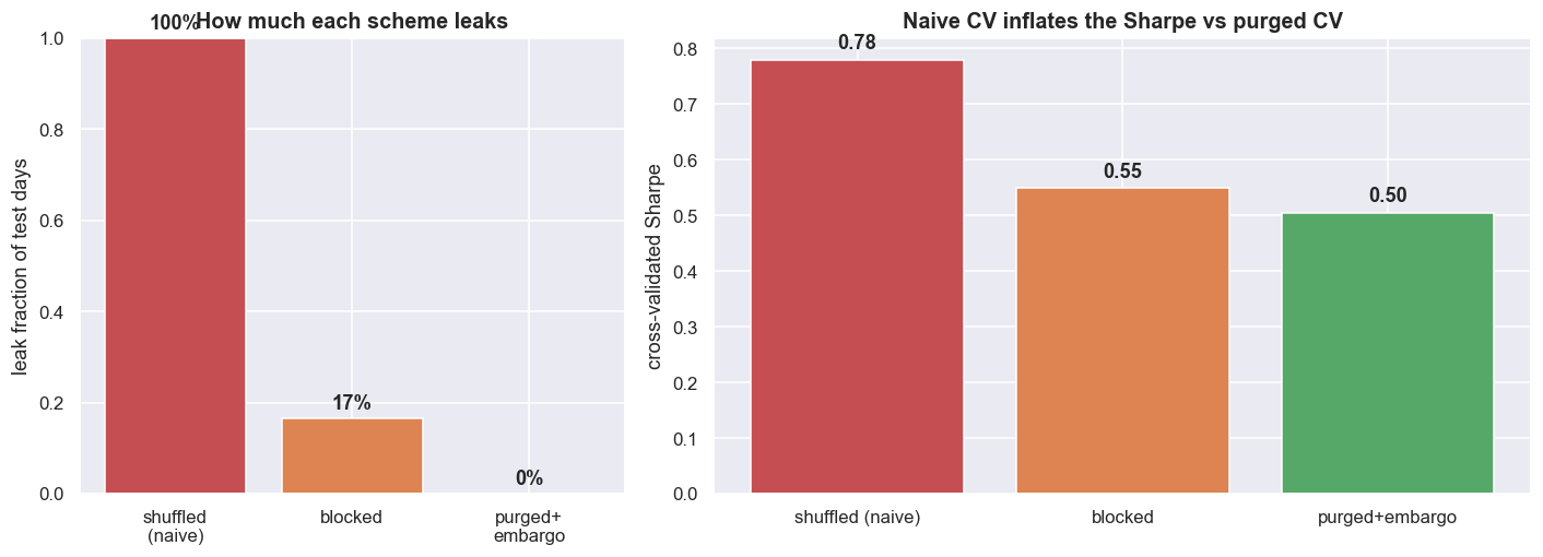
The k-fold leak is not a coding mistake you can fix with a cleaner library. It is baked into the fact that trading labels overlap in time. Shuffle the rows and you hand the model near-twins of the test set. Half the apparent cross-validated edge here was that leak, and it vanished the moment the folds were made contiguous and purged.
The Deflated Sharpe Ratio: pay a toll for every trial
Suppose you tried 64 different configurations and reported only the best one. Its Sharpe is biased upward simply because you took the maximum over many noisy tries. Even with zero true edge, the best of 64 random strategies looks good. The Deflated Sharpe Ratio (Bailey and Lopez de Prado) prices that in. Instead of comparing your Sharpe against zero, it compares it against the Sharpe you would expect to beat by luck alone after N tries. It also corrects the test for returns that are not bell-shaped.
# ---- build the grid of trials we "searched", price the best one honestly ----
entries = [1.5, 2.0, 2.5, 3.0]; exits = [-0.5, 0.0, 0.5, 1.0]; wins = [20, 40, 60, 90]
trial_cfgs = [(e, x, w) for e in entries for x in exits for w in wins]
trial_ret  = {c: daily_net(beta0, entry=c[0], ex=c[1], w=c[2]).values for c in trial_cfgs}
Rmat   = np.column_stack([trial_ret[c] for c in trial_cfgs])           # T x N matrix of daily net returns
Rmat   = np.nan_to_num(Rmat)
srd    = Rmat.mean(0) / np.where(Rmat.std(0) > 0, Rmat.std(0), np.nan)  # daily Sharpe per trial
N_TRIALS = len(trial_cfgs)
varSR  = np.nanvar(srd, ddof=1)
best   = int(np.nanargmax(srd)); r_best = Rmat[:, best]; T = len(r_best)
sr_obs = srd[best]                                                     # daily Sharpe of the selected best
sk, ku = float(skew(r_best)), float(kurtosis(r_best, fisher=False))
EG = 0.5772156649

def expected_max_sr(v, nt):
    sd = np.sqrt(v)
    return sd * ((1-EG)*norm.ppf(1 - 1.0/nt) + EG*norm.ppf(1 - 1.0/(nt*np.e)))
def psr(sr, sr_star, n, s3, k4):
    return float(norm.cdf((sr - sr_star)*np.sqrt(n-1) / np.sqrt(1 - s3*sr + (k4-1)/4*sr**2)))

sr_star   = expected_max_sr(varSR, N_TRIALS)
dsr_value = psr(sr_obs, sr_star, T, sk, ku)
psr0      = psr(sr_obs, 0.0, T, sk, ku)
sr_obs_a, sr_star_a = sr_obs*np.sqrt(ANN), sr_star*np.sqrt(ANN)

fig, (a1, a2) = plt.subplots(1, 2, figsize=(13, 4.9), gridspec_kw=dict(width_ratios=[2, 3]))
bars = a1.bar(['observed\n(best of %d)' % N_TRIALS, 'expected max\nfrom luck (SR*)', 'deflated\nexcess'],
              [sr_obs_a, sr_star_a, sr_obs_a - sr_star_a], color=[C['green'], C['amber'], C['blue']])
for bbar, v in zip(bars, [sr_obs_a, sr_star_a, sr_obs_a - sr_star_a]):
    a1.text(bbar.get_x()+bbar.get_width()/2, v+0.02, f'{v:.2f}', ha='center', fontweight='bold')
a1.axhline(0, color=C['grey'], lw=1.0); a1.set_ylabel('annualised Sharpe')
a1.set_title('Naive Sharpe vs the luck benchmark')

Ns = np.unique(np.round(np.logspace(0, 3.3, 60)).astype(int)); Ns = Ns[Ns >= 1]
dsr_curve = [psr(sr_obs, expected_max_sr(varSR, max(nt, 2)), T, sk, ku) for nt in Ns]
a2.plot(Ns, dsr_curve, color=C['purple'], lw=2.2)
a2.axhline(0.95, color=C['red'], ls='--', lw=1.2, label='0.95 credibility line')
a2.axvline(N_TRIALS, color=C['green'], ls=':', lw=1.6, label=f'N tried here = {N_TRIALS}  (DSR={dsr_value:.2f})')
a2.axvline(1, color=C['grey'], ls=':', lw=1.0)
a2.text(1.1, 0.5, f'PSR vs 0\n= {psr0:.3f}', color=C['grey'], fontsize=9, va='center')
a2.set_xscale('log'); a2.set_xlabel('number of trials N (log)'); a2.set_ylabel('Deflated Sharpe (prob true SR>0)')
a2.set_ylim(0, 1.02); a2.set_title('Significance deflates as you try more configs'); a2.legend(fontsize=9, loc='lower left')
plt.tight_layout(); plt.show()

print(f'best of {N_TRIALS} trials: daily SR {sr_obs:.3f} (ann {sr_obs_a:.2f}), skew {sk:+.2f}, kurtosis {ku:.1f}, T={T}')
print(f'against ZERO the result looks rock-solid: PSR = {psr0:.3f}.')
print(f'but the expected-max Sharpe from {N_TRIALS} lucky trials is {sr_star_a:.2f} (ann); deflating against THAT,')
print(f'the Deflated Sharpe drops to {dsr_value:.3f}. Try a few hundred configs and it falls through 0.95 entirely.')best of 64 trials: daily SR 0.070 (ann 1.11), skew +1.54, kurtosis 18.0, T=2347 against ZERO the result looks rock-solid: PSR = 1.000. but the expected-max Sharpe from 64 lucky trials is 0.56 (ann); deflating against THAT, the Deflated Sharpe drops to 0.962. Try a few hundred configs and it falls through 0.95 entirely.
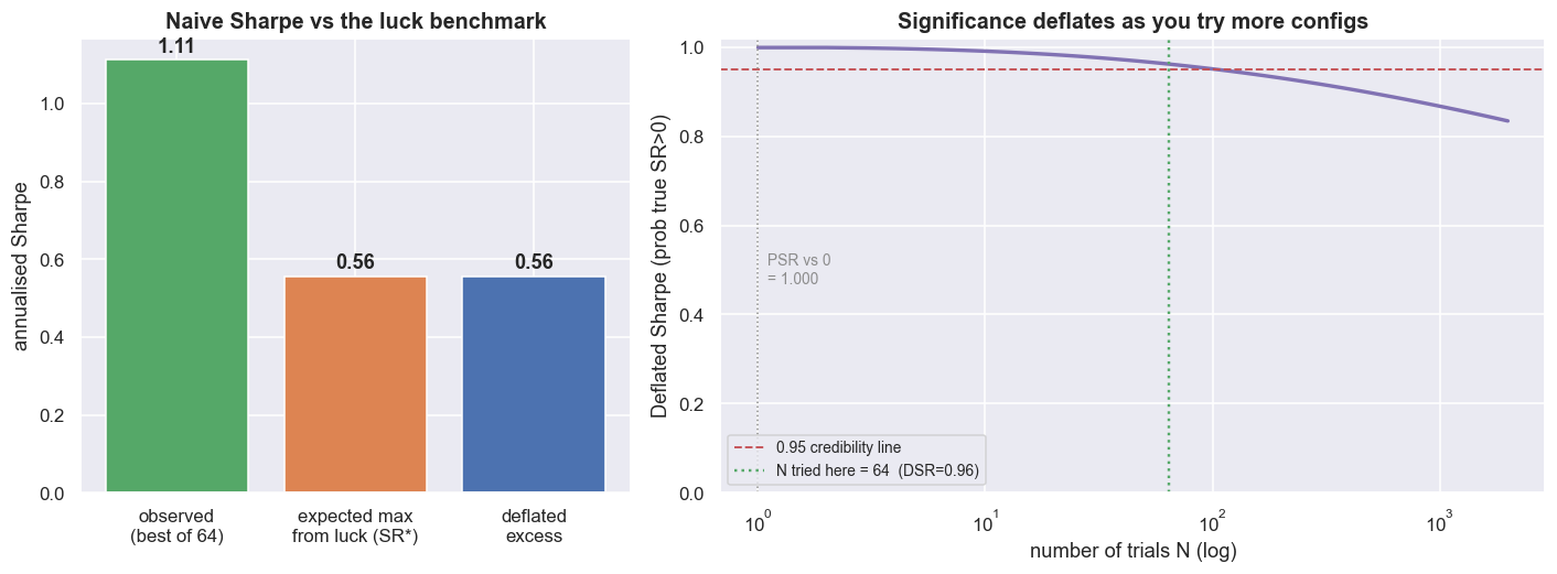
Here the best of 64 configs has a daily Sharpe of 0.070 (annualised 1.11), with returns far from bell-shaped - skew +1.54, kurtosis 18.0 - over T = 2347 days. Tested against zero, the Probabilistic Sharpe Ratio is 1.000: it looks rock-solid, all but certain. But the expected best Sharpe from 64 lucky tries is 0.56 annualised. Deflate against that benchmark instead of zero, and the Deflated Sharpe drops to 0.962. It still clears the usual 0.95 credibility line - just barely. Try a few hundred configurations instead of 64 and the same observed Sharpe falls straight through 0.95 into "not credible". The toll grows with how hard you searched.
The Deflated Sharpe here charged for 64 explicit configs. It cannot see the pairs you quietly threw away, the windows you tried last week, or the thousands of backtests in published papers you read before choosing this one. The true number of tries - and so the true haircut - is always larger than any you can write down. A PSR of 1.000 against zero means nothing unless you also say how many doors you opened to find it.
Probability of Backtest Overfitting
The Deflated Sharpe asks "is this number real?" PBO - the probability of backtest overfitting - asks the deeper question: is my whole way of picking the best config overfit? PBO is the chance that the setting which looks best in your backtest is just luck that will not repeat. We measure it with Combinatorially-Symmetric Cross-Validation (Bailey, Borwein, Lopez de Prado, Zhu). Take the T x N grid of returns from every trial, chop time into S blocks, and for every symmetric way of splitting those blocks into an in-sample half and an out-of-sample half: pick the best config in-sample, find its rank out of sample, and record where it landed. PBO is the fraction of splits where the in-sample winner falls below the out-of-sample median.
# ---- CSCV over the trial grid ------------------------------------------------
S = 8
bnds = np.linspace(0, T, S+1).astype(int)
blocks = [np.arange(bnds[i], bnds[i+1]) for i in range(S)]
def blk_sharpe(rows):
    sub = Rmat[rows]; sd = sub.std(0)
    return np.where(sd > 0, sub.mean(0)/sd, np.nan)

lams, is_best_sr, oos_sel_sr = [], [], []
for combo in itertools.combinations(range(S), S//2):
    IS = np.concatenate([blocks[i] for i in combo])
    OO = np.concatenate([blocks[i] for i in range(S) if i not in combo])
    sis, soo = blk_sharpe(IS), blk_sharpe(OO)
    nstar = int(np.nanargmax(sis))
    rank = (np.sum(soo < soo[nstar]) + 1) / (np.sum(~np.isnan(soo)) + 1)   # relative OOS rank in (0,1)
    rank = min(max(rank, 1e-3), 1 - 1e-3)
    lams.append(np.log(rank/(1-rank)))
    is_best_sr.append(sis[nstar]*np.sqrt(ANN)); oos_sel_sr.append(soo[nstar]*np.sqrt(ANN))
lams = np.array(lams)
PBO = float((lams < 0).mean())

fig, (a1, a2) = plt.subplots(1, 2, figsize=(13, 4.9))
sns.histplot(lams, bins=18, kde=True, color=C['purple'], ax=a1)
a1.axvline(0, color=C['red'], ls='--', lw=1.6)
a1.fill_betweenx([0, a1.get_ylim()[1]], a1.get_xlim()[0], 0, color=C['red'], alpha=0.08)
a1.set_title(f'CSCV logit distribution -- PBO = P(logit<0) = {PBO:.0%}')
a1.set_xlabel('logit of OOS rank of the IS-best config'); a1.set_ylabel('count of splits')

a2.scatter(is_best_sr, oos_sel_sr, s=28, color=C['amber'], edgecolor=C['grey'], alpha=0.8)
lim = [min(is_best_sr+oos_sel_sr)-0.2, max(is_best_sr+oos_sel_sr)+0.2]
a2.plot(lim, lim, color=C['grey'], ls='--', lw=1.0, label='IS = OOS')
a2.axhline(0, color=C['red'], ls=':', lw=1.0)
a2.set_xlim(lim); a2.set_ylim(lim)
a2.set_xlabel('IS Sharpe of the chosen config'); a2.set_ylabel('OOS Sharpe of that same config')
a2.set_title('In-sample winner vs its out-of-sample reality'); a2.legend(fontsize=9, loc='upper left')
plt.tight_layout(); plt.show()

print(f'CSCV: S={S} blocks, {len(lams)} symmetric splits, N={N_TRIALS} configs.')
print(f'Probability of Backtest Overfitting  PBO = {PBO:.0%}.')
print(f'median OOS Sharpe of the IS-best config: {np.median(oos_sel_sr):+.2f}  (vs its median IS Sharpe {np.median(is_best_sr):+.2f}).')
print('a PBO this high says: picking the best in-sample config is barely better than picking one at random.')CSCV: S=8 blocks, 70 symmetric splits, N=64 configs. Probability of Backtest Overfitting PBO = 54%. median OOS Sharpe of the IS-best config: +0.66 (vs its median IS Sharpe +1.25). a PBO this high says: picking the best in-sample config is barely better than picking one at random.
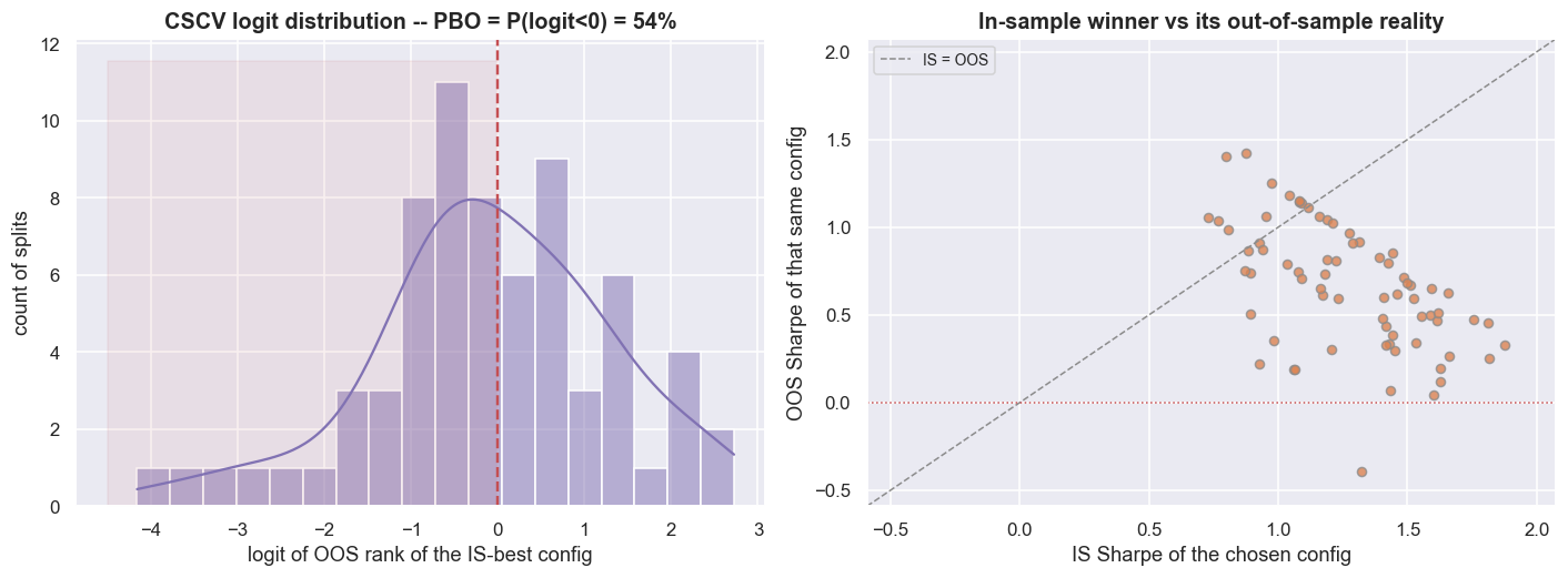
Over 70 symmetric splits of S = 8 blocks across the N = 64 configs, PBO = 54%. The config that looks best in sample lands below median out of sample more often than not - barely better than picking one at random. The scatter makes it concrete. The in-sample-best config carries a median in-sample Sharpe of +1.25, but its median out-of-sample Sharpe is just +0.66, and the cloud sprays across the diagonal instead of hugging it. Choosing the best config added almost no real out-of-sample information.
A PBO near 50% is the signature of a search that learned the noise, not the signal. It does not mean the strategy is worthless. It means the act of choosing the best config gives you essentially no edge over a coin flip. If your ranking of configs does not survive being re-ranked out of sample, you have not found a setting. You have found a story.
What survives, and how sure we are
Two questions remain. How wide is the error bar on the surviving Sharpe? And is the edge a fragile ridge or a sturdy plateau? Take the error bar first. The Sharpe is a single estimate with a fat tail, and on roughly 600 out-of-sample days that tail is wide. A block bootstrap measures it. Bootstrapping means resampling your own data many times to see how much a number wobbles. The stationary block bootstrap (Politis and Romano) resamples blocks of consecutive days - which keeps the natural clustering of real returns - a few thousand times, and reads the Sharpe off each resample.
def stationary_bootstrap_sharpe(r, B=3000, mean_block=20, seed=11):
    r = pd.Series(r).dropna().values; n = len(r); p = 1.0/mean_block
    rng = np.random.default_rng(seed)
    idxb = rng.integers(0, n, size=B); out = np.empty((B, n)); out[:, 0] = r[idxb]
    for t in range(1, n):
        restart = rng.random(B) < p
        idxb = np.where(restart, rng.integers(0, n, size=B), (idxb + 1) % n)
        out[:, t] = r[idxb]
    mu, sd = out.mean(1), out.std(1)
    return mu/np.where(sd > 0, sd, np.nan)*np.sqrt(ANN)

boot_oos  = stationary_bootstrap_sharpe(r_oos)
boot_full = stationary_bootstrap_sharpe(r_base)
ci_lo, ci_hi = np.nanpercentile(boot_oos, [2.5, 97.5])
ci_lo_f, ci_hi_f = np.nanpercentile(boot_full, [2.5, 97.5])
p_neg = float((boot_oos < 0).mean())
sr_point = sharpe(r_oos)

fig, ax = plt.subplots(figsize=(12, 5.0))
sns.histplot(boot_full, bins=60, stat='density', color=C['grey'], alpha=0.35, ax=ax, label=f'full sample (CI [{ci_lo_f:.2f}, {ci_hi_f:.2f}])')
sns.histplot(boot_oos,  bins=60, stat='density', color=C['blue'], alpha=0.55, ax=ax, label=f'out-of-sample (CI [{ci_lo:.2f}, {ci_hi:.2f}])')
ax.axvline(0, color=C['red'], lw=2.2, ls='-', label='zero')
ax.axvline(sr_point, color=C['green'], lw=2.0, ls='--', label=f'OOS point estimate {sr_point:.2f}')
ax.axvspan(ci_lo, ci_hi, color=C['blue'], alpha=0.06)
ax.set_xlabel('bootstrapped annualised Sharpe'); ax.set_ylabel('density')
ax.set_title('Stationary block bootstrap of the Sharpe -- is zero inside the interval?')
ax.legend(fontsize=9, loc='upper left')
plt.tight_layout(); plt.show()

print(f'OUT-OF-SAMPLE Sharpe {sr_point:.2f}   95% bootstrap CI [{ci_lo:.2f}, {ci_hi:.2f}]   '
      f'P(Sharpe<0) = {p_neg:.0%}')
print(f'zero is {"INSIDE" if ci_lo < 0 < ci_hi else "outside"} the interval -- we cannot reject "no edge" at 5%.')
print(f'even the full-sample CI [{ci_lo_f:.2f}, {ci_hi_f:.2f}] is wide: the point Sharpe is far less certain than it looks.')OUT-OF-SAMPLE Sharpe 0.34 95% bootstrap CI [-0.47, 1.15] P(Sharpe<0) = 20% zero is INSIDE the interval -- we cannot reject "no edge" at 5%. even the full-sample CI [0.30, 1.31] is wide: the point Sharpe is far less certain than it looks.
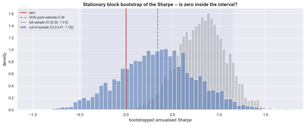
The out-of-sample point Sharpe of 0.34 comes with a 95% bootstrap interval of [-0.47, 1.15], and zero sits squarely inside it. In plain terms, we cannot rule out "no edge" at the 5% level. The chance the true Sharpe is actually negative is 20%. Even the full-sample interval, [0.30, 1.31], is wide enough that the headline number is far less certain than one clean figure ever admits. The honest read is not "Sharpe 0.34" but "somewhere between losing money one year in five and a respectable edge, and I cannot tell which from this data."
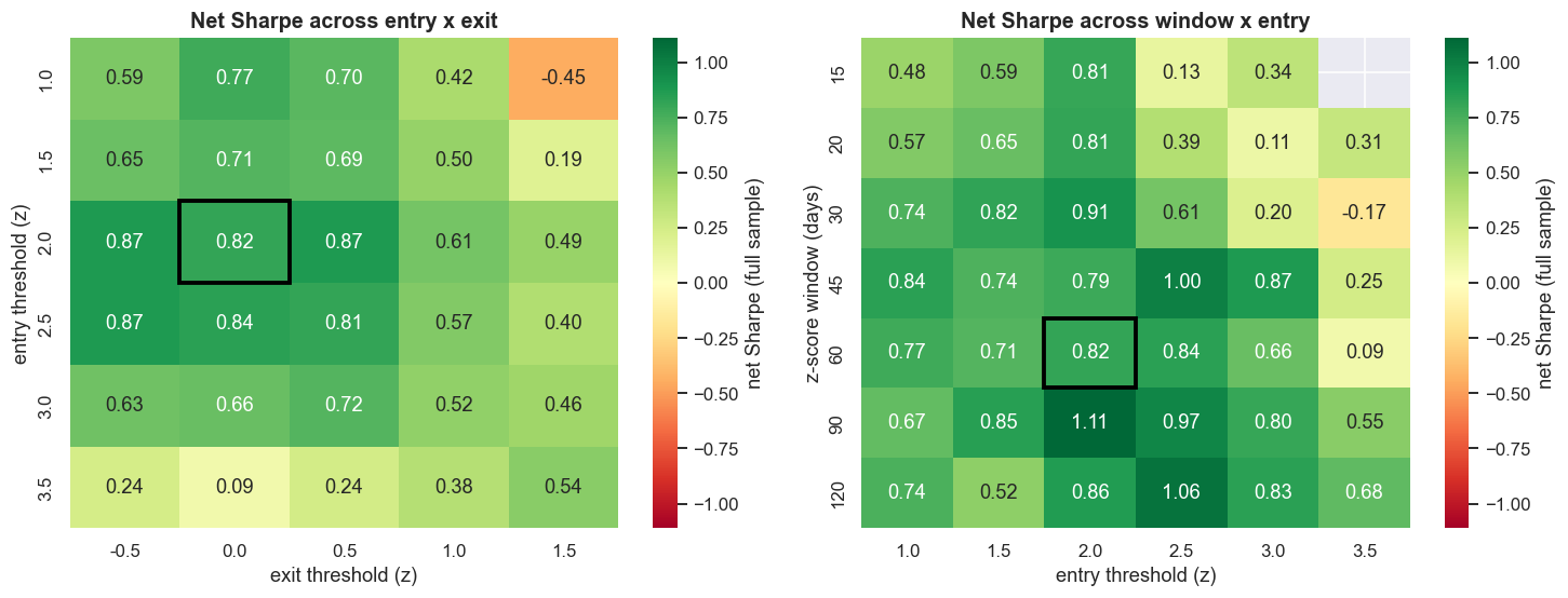
Now the shape. Picture the net Sharpe as a surface over the settings you can choose. A ridge is a thin spike - nudge a setting and the edge vanishes, a classic sign of overfitting. A plateau is a broad flat top - the edge survives across a whole neighbourhood of settings. Sweeping the net Sharpe across entry-versus-exit and window-versus-entry slices, the base config sits on a broad, gently varying plateau, not a spike. The base full-sample net Sharpe is 0.82, its 3x3 neighbourhood averages 0.79 with a standard deviation of only 0.08, and 96% of all swept cells are positive. That is the good news - the exact thresholds were not curve-fitted to a coincidence. The bad news is that it is a low plateau. The one-knob-at-a-time table shows the out-of-sample Sharpe still depends on the choices: shortening the z-score window to 90 days lifts it to 0.99, while 60 or 120 days leave it at 0.34, a tighter stop drops it to 0.19, and doubling the assumed cost takes it to 0.22. The robustness to small changes is real, but it is the robustness of a marginal edge.
def net_sharpe_cfg(entry, ex, w, sl=None):
    r = daily_net(beta0, entry=entry, ex=ex, w=w)
    return sharpe(r if sl is None else r.loc[sl])

en_ax = [1.0, 1.5, 2.0, 2.5, 3.0, 3.5]
ex_ax = [-0.5, 0.0, 0.5, 1.0, 1.5]
w_ax  = [15, 20, 30, 45, 60, 90, 120]

H1 = np.array([[net_sharpe_cfg(e, x, W) for x in ex_ax] for e in en_ax])           # entry x exit
H2 = np.array([[net_sharpe_cfg(e, EXIT, w) for e in en_ax] for w in w_ax])         # window x entry

fig, (a1, a2) = plt.subplots(1, 2, figsize=(13.5, 5.2))
vmax = np.nanmax(np.abs(np.concatenate([H1.ravel(), H2.ravel()])))
sns.heatmap(H1, ax=a1, xticklabels=ex_ax, yticklabels=en_ax, annot=True, fmt='.2f', cmap='RdYlGn',
            center=0, vmin=-vmax, vmax=vmax, cbar_kws=dict(label='net Sharpe (full sample)'))
a1.set_xlabel('exit threshold (z)'); a1.set_ylabel('entry threshold (z)'); a1.set_title('Net Sharpe across entry x exit')
a1.add_patch(plt.Rectangle((ex_ax.index(EXIT), en_ax.index(ENTRY)), 1, 1, fill=False, edgecolor='black', lw=2.5))

sns.heatmap(H2, ax=a2, xticklabels=en_ax, yticklabels=w_ax, annot=True, fmt='.2f', cmap='RdYlGn',
            center=0, vmin=-vmax, vmax=vmax, cbar_kws=dict(label='net Sharpe (full sample)'))
a2.set_xlabel('entry threshold (z)'); a2.set_ylabel('z-score window (days)'); a2.set_title('Net Sharpe across window x entry')
a2.add_patch(plt.Rectangle((en_ax.index(ENTRY), w_ax.index(W)), 1, 1, fill=False, edgecolor='black', lw=2.5))
plt.tight_layout(); plt.show()

base = net_sharpe_cfg(ENTRY, EXIT, W)
ie, ix = en_ax.index(ENTRY), ex_ax.index(EXIT)
neigh = [H1[i, j] for i in range(max(0, ie-1), min(len(en_ax), ie+2))
                  for j in range(max(0, ix-1), min(len(ex_ax), ix+2))]
neigh_mean = np.nanmean(neigh); neigh_std = np.nanstd(neigh)
frac_pos = np.mean(np.concatenate([H1.ravel(), H2.ravel()]) > 0)
print(f'base config net Sharpe {base:.2f}; its 3x3 neighbourhood mean {neigh_mean:.2f} (sd {neigh_std:.2f}).')
print(f'{frac_pos:.0%} of all swept cells have positive net Sharpe -- a broad, low ridge rather than one bright spike.')
print(f'verdict: {"PLATEAU-like (robust to small changes)" if base-neigh_mean < neigh_std+0.15 else "RIDGE-like (fragile)"}, '
f'but a low one -- robustness of a marginal edge is still a marginal edge.')base config net Sharpe 0.82; its 3x3 neighbourhood mean 0.79 (sd 0.08). 96% of all swept cells have positive net Sharpe -- a broad, low ridge rather than one bright spike. verdict: PLATEAU-like (robust to small changes), but a low one -- robustness of a marginal edge is still a marginal edge.
Put every layer on one page and the story is plain. Each ring of the funnel removed some apparent edge, and what reaches the bottom is thin and uncertain.
| Validation layer | What it asks | Result in this window |
|---|---|---|
| Single in-sample backtest | Could a rule fit the past? | Net Sharpe 1.01 |
| Walk-forward (anchored) | Survive re-estimated blind folds? | Median fold 0.47, 93% > 0, worst -0.96 |
| Walk-forward (rolling) | Same, adapting to drift | Median fold 0.57, 86% > 0, best +3.07 |
| Purged + embargoed CV | Strip the overlap leak | 0.78 -> 0.50 (55% inflation removed) |
| Deflated Sharpe (64 trials) | Beat the best of N lucky tries? | PSR-vs-0 = 1.000 collapses to DSR 0.96 |
| PBO via CSCV | Is selection itself overfit? | 54% - a coin flip |
| Block-bootstrap 95% CI | How sure is the Sharpe? | 0.34, CI [-0.47, 1.15], zero inside |
| Stability sweep | Ridge or plateau? | Plateau, 96% cells > 0, base only 0.34 OOS |
Validation working feels like a disappointment. The job of these tests is not to bless the curve. It is to subtract the part that was never real and report what is left. On this pair, what is left is a thin, uncertain, out-of-sample edge whose confidence interval includes zero. That is the method succeeding, not failing.
Where this breaks
Validation is a defence, not a guarantee. Each tool here fails quietly in its own way. An expert keeps those failure modes in view.
- Validation has its own overfitting. Run walk-forward, PBO and the rest, then tweak the strategy until they pass, and you have simply overfit to the validators instead. These tools work only when you run them once, on a hypothesis you fixed in advance. Used over and over, they become just another search that itself needs deflating.
- The number of trials is always underestimated. The Deflated Sharpe charged for 64 explicit configs. It cannot price the pairs you discarded, the windows you tried last month, or the published papers that steered you here. The true
N, and the true haircut, is larger than anything you can write down. - Purging assumes you know the holding period. We purged plus-or-minus 39 days, taken from a half-life estimate. If a spread refuses to revert and positions last longer than that, the embargo is too short and the leak survives. Purged CV controls the overlap, not the deeper drift in the relationship that walk-forward is meant to catch.
- The bootstrap assumes the past looks like the future. A block bootstrap can only reshuffle the regime you actually observed. It cannot invent the crash you never saw, the borrow squeeze, or the day the cointegration simply ends. Its interval is a floor on your uncertainty, not the whole of it.
- PBO and stability maps are relative, not absolute. A low PBO and a broad plateau only tell you that within your grid the selection is stable. They say nothing about whether the entire grid is one big pool of in-sample luck. A robust, well-validated, marginal edge is still marginal.
- None of this brings back real-world frictions. A strategy can pass every test on this page and still be untradeable once you add borrow fees, financing, position-limit bans, two-legged execution risk, and a point-in-time universe. Treat the short leg as a research abstraction unless you have a real way to implement it.
The bottom line: on HDFCBANK / KOTAKBANK, what survives walk-forward, purged cross-validation, the Deflated Sharpe, a 54% PBO, a bootstrap interval that brackets zero, and a low plateau is a thin, uncertain edge that the data cannot reliably tell apart from nothing. The rarest skill in quantitative trading is the discipline to compute all of this before you fall in love with a curve - and to walk away when the funnel comes up empty. Educational content only, not investment advice.