Implementation Pathways
What a live version actually needs: the leg vehicles, legging risk and the two-legged fill problem, impact estimated from intraday bars, participation caps, monitoring and the kill switch, and the research-to-live gap.
- ·The leg vehicles in depth
- ·Legging risk and partial fills
- ·Impact from intraday bars
- ·Participation caps and slippage
- ·Monitoring and the kill switch
- ·Retiring a strategy
Every earlier chapter handed you a research result, not a trade. You found a cointegrated spread - what's left after you subtract one stock, scaled by a hedge ratio, from another. You built a trailing z-score - how far that spread sits from its own average right now, measured in standard deviations. And you got a Sharpe ratio (return divided by risk) that stayed positive after costs on out-of-sample data: fresh data the model never saw while it was built. None of that is a position. The distance between a result that passed your tests and a real book on NSE is not one decision. It is a whole chain of them, and most of the ways to lose money hide in that chain, not in the signal.
This chapter is the unglamorous machinery behind that chain. Which vehicle holds each leg. What it costs you when your two orders can't fill at the same instant - that gap is legging risk. How wide the trading spread and the price impact of your own order really are when you measure them from bars instead of guessing. And the monitoring, the kill switch, and the discipline to retire a strategy once its edge is gone. Nothing here sends an order. This is education about implementation, not a recipe for placing trades. The point is simple: a statistical relationship is not a tradable edge, and even a tradable edge dies without this scaffolding.
The pipeline is a loop, not a launch button
Beginners build the left half of the system - data, signal, backtest - and skip the right half. The right half is the part that keeps you solvent. Think of implementation as a loop, not a one-time launch. A result that makes money after costs picks a vehicle for each leg. The vehicle sets how you execute: legging, slippage (the gap between the price you expected and the price you got), how much of the volume you take, and when you square off. Execution feeds monitoring: the running spread, the z-score, your exposure, your profit and loss. And monitoring makes one of two calls. It keeps the trade on, or it retires the trade and sends the idea back to research - never straight back to the order book.
Picking the vehicle: how long you hold decides
The long leg is easy. You buy the cash stock for delivery and hold it. The hard part is the short leg - the stock you sell. Here you have three honest choices, and each is a trade-off you make on purpose, not a default. Cash intraday costs nothing to hold overnight, but the rules force you to close it near 3:20pm. So you pay the full spread to get out, then pay it again the next morning to get back in, just to stay in the trade. SLB-borrowed stock (stock you borrow so you can sell it short) charges a borrow fee that is lumpy and scarce. Many stocks have no borrow at all, and the fee can spike into double digits exactly when everyone wants the same short. Stock futures are the workhorse: you pay to enter and exit once, carry a small running cost, roll to the next contract every expiry, and carry a basis - the gap between the future and the spot price - that wobbles around.
The variable that decides it is how long you must hold. Intraday re-crossing is a straight ramp upward. The vehicles you pay once start higher but barely grow. Price the crossover straight from the cost model and the picture is stark: with a per-round-trip transaction cost of about 28 bps (four fills - two legs, entered and exited), intraday re-crossing overtakes futures after roughly one day of holding.
# Carry-cost crossover: total round-trip cost (bps of leg notional) vs holding period.
# Uses the COST model. Spread/impact defaults are validated against real 5m data later.
days = np.arange(1, 121)

# one full entry+exit round trip for a PAIR (4 fills), as bps of one leg's notional
rt_pair_bps = pair_roundtrip_cost_frac("MIS") * 1e4          # ~ statutory + spread + impact, x4
roll_bps    = pair_roundtrip_cost_frac("MIS") * 1e4 * 0.5    # a futures roll ~ half a full round trip
slb_fee_ann = 0.03                                           # 3%/yr representative borrow fee (lumpy!)
fut_fin_ann = 0.0                                            # net financing ~neutral for a short (r approx q effect)

# Intraday: you cannot hold overnight, so to *carry* H days you re-establish the pair each day.
cost_intraday = rt_pair_bps * days
# SLB: pay one round trip, then borrow fee accrues on both legs' notional.
cost_slb = rt_pair_bps + slb_fee_ann * 1e4 * days / 365.0
# Futures: pay one round trip, then a roll every ~30 days, plus ~neutral financing.
cost_fut = rt_pair_bps + roll_bps * (days / 30.0) + fut_fin_ann * 1e4 * days / 365.0

fig, ax = plt.subplots(figsize=(11, 4.8))
ax.plot(days, cost_intraday, color=C["red"],   lw=2.2, label="Cash intraday (re-cross daily)")
ax.plot(days, cost_slb,      color=C["green"], lw=2.2, label="SLB borrow (3%/yr fee)")
ax.plot(days, cost_fut,      color=C["blue"],  lw=2.2, label="Stock futures (monthly roll)")
ax.set_ylim(0, np.percentile(cost_intraday, 60))
ax.set_title("Cost of CARRYING a pair vs holding period (bps of leg notional)")
ax.set_xlabel("intended holding period (calendar days)"); ax.set_ylabel("cumulative round-trip cost (bps)")
ax.legend(loc="upper left")
plt.tight_layout(); plt.show()

x_cross = days[np.argmin(np.abs(cost_intraday - cost_fut))]
print(f"one pair round trip ~ {rt_pair_bps:,.0f} bps (4 fills: 2 legs x entry+exit)")
print(f"intraday re-crossing overtakes futures after ~{x_cross} day(s) of holding.")
print("Read: intraday is ONLY for sub-day pairs; for any multi-day hold, futures/SLB dominate.")one pair round trip ~ 28 bps (4 fills: 2 legs x entry+exit) intraday re-crossing overtakes futures after ~1 day(s) of holding. Read: intraday is ONLY for sub-day pairs; for any multi-day hold, futures/SLB dominate.
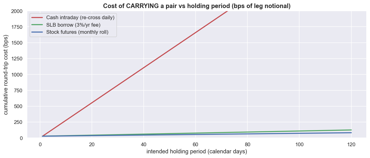
The holding period picks the vehicle, not your preference. A signal that reverts within the day can use cash intraday. Anything you hold for days or weeks must use futures or SLB. Most cointegration trades are in this second group, because their half-life - the time a deviation takes to shrink by half, and so the natural holding period - runs to several days. Paying the full spread twice a day just to stay in a multi-week trade is ruinous. The futures line includes a roll roughly every 30 days. But its real enemy is not this trading cost. It is the basis wobble and the lot-size rounding that the price series never showed you.
That last point is the quiet killer. You estimate the hedge ratio - how many units of one stock you trade against the other so their shared market moves cancel - on cash closing prices. But you trade it in futures that sit off the spot price, round to fixed lot sizes, and carry an expected dividend the cash series already stripped out. Each one is a small, built-in gap between the spread you backtested and the spread you actually trade. It is always there. It is not random noise you can diversify away.
Legging risk: two orders that must both happen
In a backtest, both legs fill on the same bar at the same price. Reality is messier. You send leg A and leg B. One fills first. In the gap before the other fills, the market moves. That gap is legging risk. It causes four separate failures. First, slippage on the second leg as the price drifts away while you chase it. Second, partial fills that leave you off your target ratio. Third, a hedge-leg failure: one leg fills, the other is rejected or untradeable, and now you hold a one-sided directional bet - the very risk the pair was meant to remove. Fourth, an outright rejection from margin, a price band, a freeze quantity, or an F&O ban.
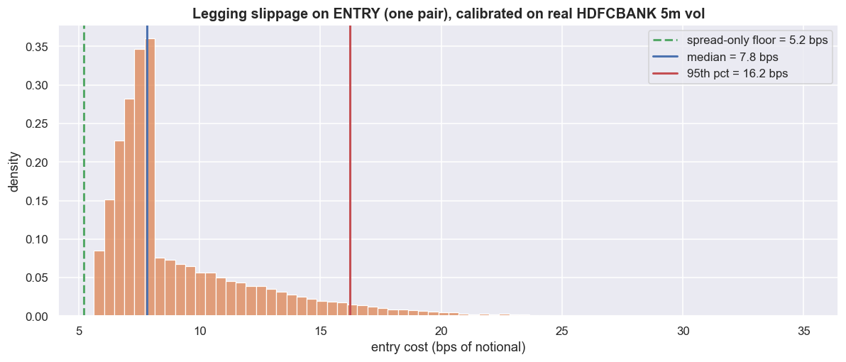
Put a number on it with a simulation built from real intraday data. The measured 5-minute return volatility is 13.1 bps, which works out to about 0.757 bps per second that you sit unhedged. Run thousands of legged entries against a spread-only floor of 5.2 bps, and the costs do not sit at that floor. The median legged entry costs 7.8 bps. The 95th-percentile fill costs 16.2 bps - a bad-gap fill at several times the spread. And 24% of entries cost more than twice the spread floor. The spread of outcomes leans heavily to the expensive side, because the gap drift is random but you always chase into the move. And this is the entry only. The exit legs the same way, doubling the legging drag over a full round trip.
# Two-leg fill slippage, simulated and CALIBRATED ON REAL 5m INTRADAY VOLATILITY.
# We measure how fast a liquid name moves intra-bar, then ask: if leg B fills g seconds
# after leg A, how much extra cost does that gap add beyond just crossing the spread?
cal = load("HDFCBANK", interval="5m", start="2026-04-01", end="2026-06-26", source="db")
r5 = np.log(cal["close"] / cal["close"].shift(1))
same = pd.Series(cal.index.date, index=cal.index)
r5 = r5[same.values == same.shift(1).values].dropna()          # drop overnight gaps
vol_per_sec = r5.std() / np.sqrt(300)                           # a 5-minute bar = 300 seconds
half_spread = 5.2 / 2 / 1e4                                     # ~5.2 bps full spread (measured below), as a fraction

rng = np.random.default_rng(7)
N = 40000
gap = rng.uniform(2, 90, N)                                     # seconds to fill the 2nd leg while chasing
z   = rng.standard_normal(N)
drift_sd     = vol_per_sec * np.sqrt(gap)                       # std of leg-B move over the gap
directional  = drift_sd * z                                    # signed move on leg B (mean 0, adds variance)
adverse_bias = 0.40 * drift_sd                                 # systematic: you tend to chase INTO the move
spread_only  = 2 * half_spread                                 # both legs cross half the spread - unavoidable
legging_cost = (spread_only + adverse_bias + np.abs(directional) * (directional > 0)) * 1e4  # bps, entry
# (we keep only the adverse half of the directional move; a favourable move just lowers cost toward spread-only)

fig, ax = plt.subplots(figsize=(11, 4.8))
sns.histplot(legging_cost, bins=70, color=C["amber"], stat="density", ax=ax)
ax.axvline(spread_only * 1e4, color=C["green"], lw=2, ls="--", label=f"spread-only floor = {spread_only*1e4:.1f} bps")
ax.axvline(np.median(legging_cost), color=C["blue"], lw=2, label=f"median = {np.median(legging_cost):.1f} bps")
ax.axvline(np.percentile(legging_cost, 95), color=C["red"], lw=2, label=f"95th pct = {np.percentile(legging_cost,95):.1f} bps")
ax.set_title("Legging slippage on ENTRY (one pair), calibrated on real HDFCBANK 5m vol")
ax.set_xlabel("entry cost (bps of notional)"); ax.set_ylabel("density"); ax.legend()
plt.tight_layout(); plt.show()

print(f"measured 5m return vol = {r5.std()*1e4:.1f} bps  ->  per-second vol = {vol_per_sec*1e4:.3f} bps")
print(f"spread-only floor  : {spread_only*1e4:5.1f} bps")
print(f"median legged entry: {np.median(legging_cost):5.1f} bps")
print(f"95th-pct legged    : {np.percentile(legging_cost,95):5.1f} bps  (a bad-gap fill)")
print(f"share of entries costing > 2x the spread floor: {(legging_cost > 2*spread_only*1e4).mean():.0%}")
print("And this is ENTRY only - the exit legs the same way, doubling the legging drag over a round trip.")measured 5m return vol = 13.1 bps -> per-second vol = 0.757 bps spread-only floor : 5.2 bps median legged entry: 7.8 bps 95th-pct legged : 16.2 bps (a bad-gap fill) share of entries costing > 2x the spread floor: 24% And this is ENTRY only - the exit legs the same way, doubling the legging drag over a round trip.
Your two defences pull in opposite directions. Market orders guarantee both legs fill, but you pay the full chase. Limit orders cap the slippage, but they raise the chance that leg B never fills - the worse outcome, because it leaves you naked. And being naked is not a rounding error. Even at a generous 95% per-leg fill probability you still end up unhedged about 9.5% of the time - one trade in ten. At 90% per leg it rises to 18%. That is not a small directional bet. It is a full single-stock position the strategy never planned to hold.
The most expensive outcome in pairs trading is not slippage. It is being unhedged. A 95%-reliable fill on each leg still leaves you naked roughly one entry in ten, and that tail never shows up in a slippage chart. The simulation can price the gap. It cannot price the case where leg B is simply unavailable - no borrow, an F&O ban, a locked circuit - and you sit directional in a position you never wanted.
Costs you can least defend: spread and impact
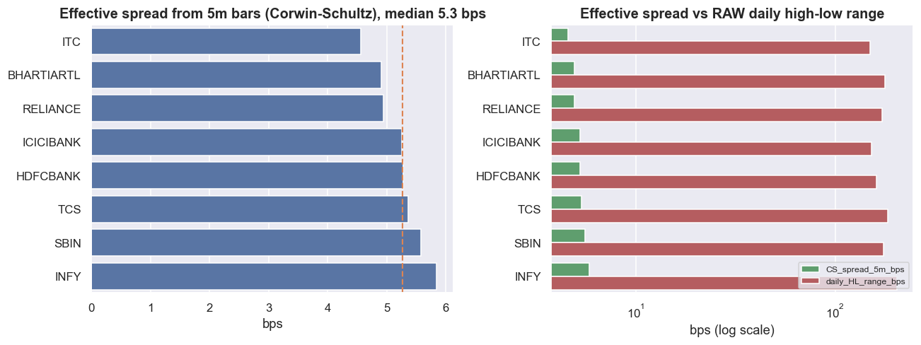
So far the cost model has used assumed values for two things: the half-spread (half the gap between the best buy and sell price, which you cross to trade right now) and the impact (how much your own order pushes the price). These are the two numbers you can least defend ahead of time, because they shift with your size, the time of day, and how the order book looks when you trade. So measure them instead of guessing. OHLCV bars carry no quoted bid-ask, so estimate the effective spread with the Corwin-Schultz high-low estimator, which backs out the bid-ask from the range of consecutive bars. Across the liquid large-caps the effective spread clusters tightly: 4.6 to 5.8 bps, with a representative median around 5.3 bps. When you have no intraday data, the naive fallback is the daily high-low range. It is wrong by a huge margin - about 33 times the effective spread - because it stuffs the whole day's volatility into "spread".
# Visualise the measured effective spread, and how crude the daily-range fallback is.
fig, axes = plt.subplots(1, 2, figsize=(12, 4.6))
sp = spreads.reset_index()
sns.barplot(data=sp, y="symbol", x="CS_spread_5m_bps", color=C["blue"], ax=axes[0])
axes[0].axvline(cs_repr, color=C["amber"], ls="--", lw=1.4)
axes[0].set_title(f"Effective spread from 5m bars (Corwin-Schultz), median {cs_repr:.1f} bps")
axes[0].set_xlabel("bps"); axes[0].set_ylabel("")
m = sp.melt(id_vars="symbol", value_vars=["CS_spread_5m_bps","daily_HL_range_bps"],
            var_name="measure", value_name="bps")
sns.barplot(data=m, y="symbol", x="bps", hue="measure",
            palette={"CS_spread_5m_bps": C["green"], "daily_HL_range_bps": C["red"]}, ax=axes[1])
axes[1].set_title("Effective spread vs RAW daily high-low range")
axes[1].set_xlabel("bps (log scale)"); axes[1].set_ylabel(""); axes[1].set_xscale("log")
axes[1].legend(title="", loc="lower right", fontsize=8)
plt.tight_layout(); plt.show()
print("The daily high-low range is a usable LAST-RESORT proxy when intraday is missing, but it bundles")
print("the whole day's volatility into 'spread' and is wrong by an order of magnitude. Prefer real bars.")The daily high-low range is a usable LAST-RESORT proxy when intraday is missing, but it bundles the whole day's volatility into 'spread' and is wrong by an order of magnitude. Prefer real bars.
Impact is the other half. Model it as a square-root rule: the price moves roughly as the square root of how much of the bar's volume you grab. Calibrated on each stock's daily volatility, that comes to about 8.3 bps at 1% participation, 18.5 bps at 5%, and 26.1 bps at 10%. The curve bends over: doubling your size does not double the impact, but the impact never stops growing either.
# Square-root market impact: bigger orders move the price ~ sqrt(participation).
name = "RELIANCE"
dd = load(name, interval="D", start="2024-06-01", end="2026-06-26")
daily_vol_bps = np.log(dd["close"]).diff().std() * 1e4          # daily return vol, from real data
Y = 0.6                                                          # square-root-law coefficient (~0.3-1 in the literature)
part = np.linspace(0.002, 0.20, 200)                            # order as a fraction of ADV
impact = Y * daily_vol_bps * np.sqrt(part)
cap = 0.10                                                      # our participation cap: never exceed 10% of volume
impact_at_cap = Y * daily_vol_bps * np.sqrt(cap)

fig, ax = plt.subplots(figsize=(11, 4.8))
ax.plot(part*100, impact, color=C["purple"], lw=2.4)
ax.axvline(cap*100, color=C["red"], ls="--", lw=1.6, label=f"participation cap = {cap:.0%}")
ax.scatter([cap*100], [impact_at_cap], color=C["red"], zorder=5)
ax.set_title(f"{name}: modelled market impact vs participation (daily vol {daily_vol_bps:.0f} bps)")
ax.set_xlabel("order size as % of volume traded"); ax.set_ylabel("price impact (bps)"); ax.legend()
plt.tight_layout(); plt.show()
for pv in (0.01, 0.05, 0.10):
    print(f"at {pv:4.0%} participation -> impact ~ {Y*daily_vol_bps*np.sqrt(pv):4.1f} bps")
print("Impact is convex-down: doubling size does NOT double impact, but it never stops growing either.")at 1% participation -> impact ~ 8.3 bps at 5% participation -> impact ~ 18.5 bps at 10% participation -> impact ~ 26.1 bps Impact is convex-down: doubling size does NOT double impact, but it never stops growing either.

That bend is the whole argument for a participation cap - a hard rule never to take more than X% of a bar's volume. A reusable slippage function that charges spread plus impact on each fill shows the trade-off: about 10.4 bps per fill at a 1% cap, 27.3 bps at 10%. A tight cap (2-5%) protects your price but stretches the exit across more bars. And a long, slow exit is exactly when a circuit, a gap, or a borrow recall can trap you mid-unwind. A loose cap (10-20%) gets you flat fast but pays the steep impact and signals your hand to the market. No single setting is both cheap and fast.
Now put it all into one honest number. A pair round trip is four fills. Each fill pays statutory charges, half the measured spread, and the modelled impact at the participation cap. Add them up and the total round-trip cost is about 123 bps - 1.23% of one leg's notional. That is the hurdle every signal must clear before you earn a single rupee of edge. If your backtested edge per trade is, say, 30 to 50 bps, this one number decides whether the strategy lives or dies.
Every cost here is an estimate, and estimates tend to flatter you. The Corwin-Schultz spread is inferred from OHLC, not quoted. The impact model is a square-root assumption with a coefficient you picked. The legging volatility comes from one stock's recent tape. When the hurdle adds up to 123 bps and a plausible per-trade edge is only 30 to 50 bps, the right question is not "is it profitable?" It is "how wrong can my cost estimate be before the profit turns into a loss?" And the answer is: not very wrong at all.
Monitoring and the kill switch
A managed pair is not something you set and forget. The smallest workable system is a short pipeline. A data feed drives a signal engine. Every order passes a risk-and-limits gate before it reaches the order path. And a monitoring loop watches the running state - spread, z-score, exposure, profit and loss, a check that both legs are on, and margin headroom - with a kill switch wired straight to a flatten action. A kill switch is a pre-decided rule, plus a button, that closes everything at once.
The kill switch is not a vague plan to "keep an eye on it." It is a small set of rules decided in advance, and any one of them flattens the book. Build it as pure logic that decides but never sends an order. The gates check on every tick. A healthy pair returns OK. A spread blow-out past a hard limit (in the sample, |z| = 4.8) returns FLATTEN, because the relationship may have broken rather than snapped back. A broken leg returns FLATTEN, because a naked single-stock position has to go right now.
Before any of this reaches a broker, the whole loop runs in sandbox trading (analyzer mode in OpenAlgo). The same code path simulates fills and returns order objects without sending anything. The order path comes in two shapes. One is a plain order per leg, carrying a product (MIS intraday or NRML carry) and a price_type (MARKET or LIMIT). The other is a smart order that reconciles a symbol to a target position size, and can be sent again safely without doubling up - the natural fit for a pair that must hold a neutral ratio and then be flattened to zero. We describe the function signatures only. Nothing here is an instruction to place a trade.
A kill switch is only as good as the data feed and the discipline behind it. A stale tick, a missed alert, or a single human override "just this once" defeats the whole thing. The intraday square-off clock is the same kind of hard rule. Flatten on your schedule, before the forced square-off window - never at the market's worst liquidity on someone else's clock. The switch must be mechanical and decided in advance, or it is just decoration.
Retiring a strategy when the edge dies
The hardest gate has no dramatic trigger. It is a slow death. An edge wears away as others find it, as the relationship weakens, as costs creep up. Take a real pair. Fix the hedge ratio on the early window (here beta = 1.08 over the first two years). Then watch the rolling co-movement and the spread's stability fall apart. The diagnosis is blunt: the 120-day return correlation spends 48% of the history below 0.5. Nearly half the time, the two stocks are not even moving together at the level the trade assumed. When co-movement spends long stretches under your threshold, and the spread keeps widening instead of reverting, the relationship that justified the pair is decaying.
# Edge decay on a REAL pair: rolling co-movement and rolling spread stability.
a, b = "HDFCBANK", "KOTAKBANK"
pa, pb = load(a)["close"], load(b)["close"]
df = pd.concat([np.log(pa), np.log(pb)], axis=1).dropna(); df.columns = [a, b]
train = df[df.index < df.index[0] + pd.Timedelta(days=730)]            # fix the hedge ratio on first 2 yrs
beta = np.polyfit(train[b], train[a], 1)[0]
spread = df[a] - beta * df[b]
z = (spread - spread.rolling(120).mean()) / spread.rolling(120).std()
roll_corr = df[a].diff().rolling(120).corr(df[b].diff())               # 120d rolling return correlation
roll_sd   = spread.rolling(120).std()                                  # spread instability

fig, axes = plt.subplots(2, 1, figsize=(11.5, 7), sharex=True)
axes[0].plot(roll_corr.index, roll_corr, color=C["blue"], lw=1.6, label="120d rolling return corr")
axes[0].axhline(0.5, color=C["red"], ls="--", lw=1.3, label="retire-watch threshold (0.5)")
axes[0].fill_between(roll_corr.index, 0, 1, where=(roll_corr < 0.5), color=C["red"], alpha=0.12)
axes[0].set_ylim(0, 1); axes[0].set_title(f"{a} vs {b}: co-movement is NOT constant - monitor it")
axes[0].set_ylabel("rolling corr"); axes[0].legend(loc="lower left", fontsize=8)
axes[1].plot(roll_sd.index, roll_sd, color=C["amber"], lw=1.6)
axes[1].set_title("Rolling spread volatility - a widening spread is an edge under stress")
axes[1].set_ylabel("rolling std of spread"); axes[1].set_xlabel("")
plt.tight_layout(); plt.show()

frac_weak = (roll_corr < 0.5).mean()
print(f"hedge ratio (fixed on first 2y): beta = {beta:.2f}")
print(f"share of history with 120d return-corr below 0.5: {frac_weak:.0%}")
print("When co-movement spends long stretches below your threshold and the spread keeps widening, the")
print("relationship that justified the pair is decaying. Retire it - a dead edge bleeds costs every trade.")hedge ratio (fixed on first 2y): beta = 1.08 share of history with 120d return-corr below 0.5: 48% When co-movement spends long stretches below your threshold and the spread keeps widening, the relationship that justified the pair is decaying. Retire it - a dead edge bleeds costs every trade.
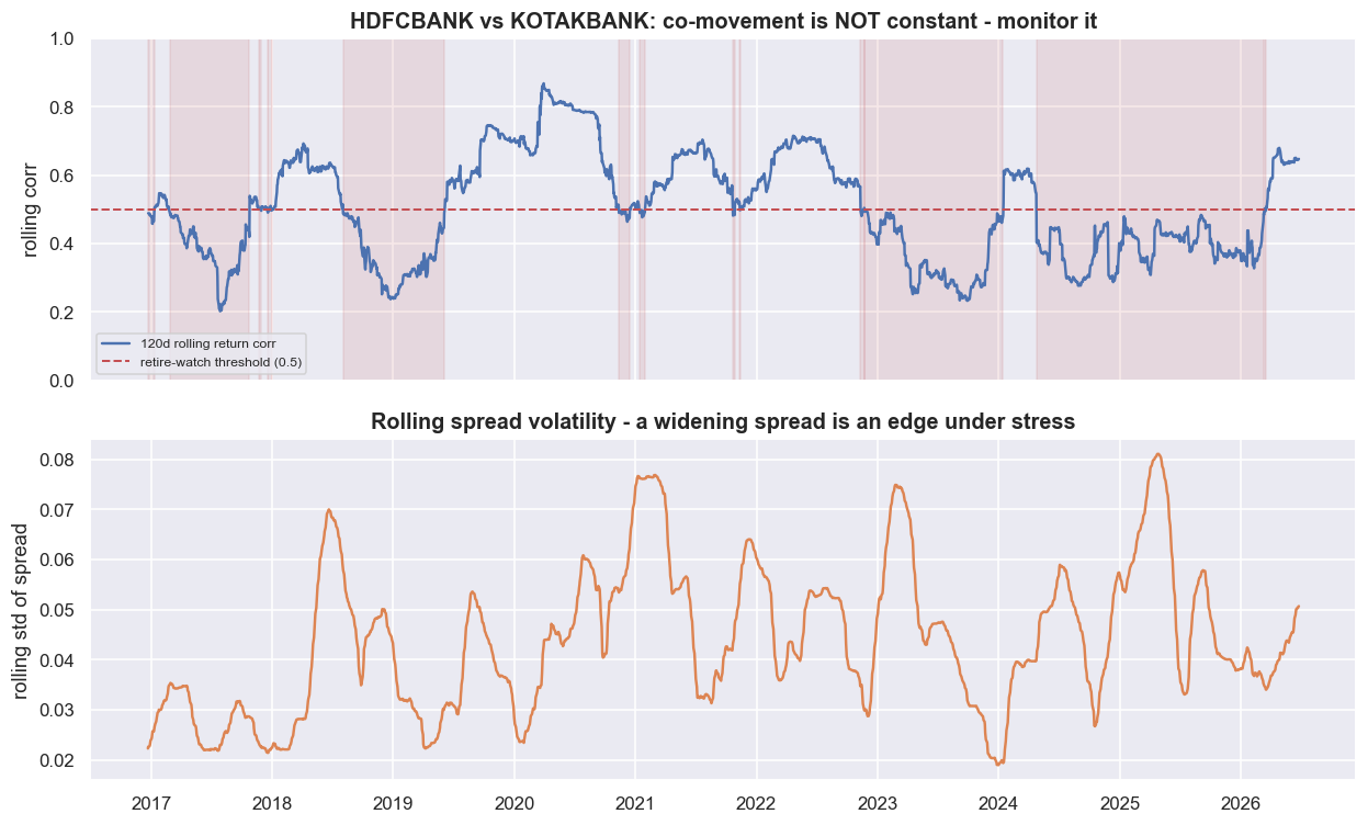
The right move is not to size up and "wait for reversion." That is the gambler's move - doubling into a dead edge while it bleeds 123 bps every round trip. The right move is to retire the strategy and send the idea back to research. The data makes the call, not your hope. That is the loop closing: monitoring spotted the decay, the retire gate fired, and the idea goes back to research, not to the order book.
Where this breaks
- Every cost here is an estimate, and estimates run optimistic. The Corwin-Schultz spread is inferred from OHLC, not quoted. The impact model is a square-root assumption with a coefficient you chose. The legging simulation is calibrated on one stock's recent 5-minute volatility. Real fills in thin stocks, a fast tape, or a stressed market are worse - sometimes far worse. The 123 bps hurdle is the floor, not the ceiling.
- The legging simulation assumes you always get both legs. It prices the slippage of a gap, not the case where leg B is simply unavailable - no borrow, an F&O ban, a locked circuit - and you sit naked. A 95% per-leg fill still leaves you naked roughly one trade in ten, and that tail is in none of the charts above.
- The carry-cost crossover hides how scarce borrow really is. The SLB line uses one tidy fee. In practice, borrow is lumpy, can be recalled mid-trade, and is missing for exactly the stocks you most want to short. The futures line ignores margin financing and gap-day margin calls that can force you to cut at the worst moment, plus the built-in tracking error from basis, lot rounding, and dividends.
- The kill switch and monitoring are only as good as the feed and the discipline behind them. A stale tick, a missed alert, or a human override defeats the whole thing. The switch must be mechanical and decided in advance, or it is just decoration.
- No backtest, however honest, equals a real track record. The gap between research and reality - queue position, partial fills, rejections, latency, basis, recalls, regime change - only shows up with small size, in sandbox first. Sandbox results are a hypothesis about execution, not proof of it.
The final, honest word: a statistical relationship is not a tradable edge, and a tradable edge, once found, does not last forever. What stands between a clean research curve and a surviving book is the unglamorous machinery of this chapter - the right vehicle, controlled legging, measured costs, hard participation caps, square-off discipline, monitoring, a kill switch decided in advance, and the maturity to retire a strategy once its edge is gone. Build that machinery, or do not trade the edge at all. Educational content only, not investment advice.