Stationarity and Random Walks

A stock falls for three weeks, and somewhere a trader says the words that have funded more blown accounts than any other: "it's oversold, it has to revert." Stop there. Before you can say a series reverts, you have to show it has something to revert to. That means a fixed average and a stable spread of values that the next price is tied to. Most price series have neither.

The whole of statistical arbitrage rests on one property: stationarity. A stationary series wanders around a fixed average and keeps getting pulled back to it - the opposite of a price that drifts off forever. Stationarity is what decides whether "it will revert" is a real, tradeable statement or just a story you are painting onto a chart. This chapter shows, on real NSE data, that a single stock price almost never has it - and that its returns almost always do. That gap is not a curiosity. It is the reason stat-arb never trades a price, only a spread it has built to be stationary.

A quick statistics primer for time-series traders

Every test in this course leans on a handful of statistics ideas. Here they are in one place, in plain words. If you have seen them before, skim. If not, this is the vocabulary the rest of the course assumes, and the few minutes here will save you a lot of confusion later.

• Sample vs population. The population is every value that could ever occur; the sample is the finite slice you actually measured. You never see the population. Every number you compute - a mean, a correlation, a p-value - is a guess about the population made from one sample, and a different sample would give a slightly different answer.
• Mean, variance, standard deviation. The mean is the average. The variance is the average squared distance from the mean; the standard deviation (its square root) is the typical distance from the mean, in the same units as the data. Most of the risk numbers in this course are just standard deviations of something.
• Z-score. How many standard deviations a value sits from its mean: z = (value - mean) / sd. A z of +2 means "two standard deviations above average." Our entire trade signal is just the z-score of the spread.
• Standard error. The standard deviation of an estimate, not of the data. Measure the mean from 50 points, redo it on another 50, and it jumps around; the standard error is how much. It shrinks as the sample grows (roughly like one over the square root of the sample size). Small samples give jumpy estimates - keep that in mind every time a result rests on a short window.
• Null and alternative hypothesis. A test sets up a boring default, the null (for example, "this series is a random walk"), and a claim you would need evidence for, the alternative ("it mean-reverts"). The test asks whether the data is surprising enough under the null to abandon it.
• P-value, stated carefully. The p-value is the chance, if the null hypothesis were true, of seeing a result at least as extreme as the one you got. Small (below your threshold, usually 0.05) means the data would be surprising under the null, so you reject the null. It is not the probability that the null is true, and not the probability that your finding is real. It measures only surprise under the null.
• Confidence interval. A range built so that, with a stated confidence such as 95%, the method captures the true value most of the time. "Half-life 24 days, 95% interval [12, 60]" means the best estimate is 24, but the data is consistent with anything from 12 to 60. A wide interval is a warning that you know far less than the single number suggests, so report intervals, not just point estimates.
• Type I and Type II errors. A Type I error is a false positive: you reject the null when it was true (you "find" a pair that is not there). A Type II error is a false negative: you keep the null when the alternative was true (you miss a real pair). Lowering your p-value threshold cuts Type I errors but raises Type II.
• Statistical power. The chance a test correctly rejects a false null - that is, catches a real effect. Power rises with sample size and with the strength of the effect. Low-power tests miss real effects, and they also make the positives they do report less trustworthy.
• Multiple testing. Run one test at the 5% level and a false positive is rare. Run 500 and you expect about 25 false positives by luck alone. Searching a whole universe for pairs is exactly this trap, and Chapter 8 is about escaping it.
• Why time-series tests are weaker. Classic statistics assumes independent observations. Daily prices are anything but - today is glued to yesterday. That memory means a 2,000-day series carries far less independent information than 2,000 coin flips, so time-series tests like ADF have low power: they need a lot of data to be sure, and they are easy to fool on short or regime-shifting samples. Treat every single test as weak evidence, and trust only what also survives out of sample.

With that vocabulary in hand, here is the one property everything rests on.

The one idea: I(1) prices, I(0) returns

A series is integrated of order d - written I(d) - if you have to difference it d times before it becomes stationary. ("Difference" just means take the change from one step to the next.) Two orders matter for everything that follows.

An I(1) series - a price - needs differencing once. The level itself has a unit root, which is the formal way of saying it behaves like a random walk: it wanders with no average to return to, and the range of where it might be keeps growing as time passes. Ask "where should this price be?" and there is no honest answer. An I(0) series - a return - is already stationary. It has a fixed long-run average (near zero for daily log returns), a finite and roughly steady spread of values, and almost no memory from one day to the next. Any move away from its average is temporary by design. The one operation that turns a price into a return is the log difference, r_t = log(P_t) - log(P_{t-1}). That is the whole reason returns, not prices, are the well-behaved object - and the reason the only tradeable mean-reverting object here is never a price, but a spread you build and force to be I(0).

A random walk and a mean-reverter, built from scratch

Before touching market data, build both objects yourself so there is no doubt about what "stationary" looks like. A random walk is x_t = x_{t-1} + e_t: tomorrow's value is today's value plus fresh random noise, and that noise stays in the level forever. This is the textbook I(1) process and the standard model of an efficient price. A stationary AR(1) is y_t = phi * y_{t-1} + e_t with |phi| < 1. AR(1) means each step leans back toward the average; here a shock fades away step by step at rate phi, so the series keeps getting pulled back toward zero. That is I(0), and the standard model of a mean-reverting spread.

Copy

rng = np.random.default_rng(2)        # seeded: fully reproducible
n = 1500
eps = rng.standard_normal(n)          # white noise, the shocks
rw  = np.cumsum(eps)                  # random walk  x_t = x_{t-1} + e_t   -> I(1)
phi = 0.85
ar  = np.zeros(n)                     # stationary AR(1)  y_t = phi y_{t-1} + e_t -> I(0)
for t in range(1, n):
    ar[t] = phi * ar[t-1] + eps[t]

fig, ax = plt.subplots(2, 2, figsize=(13, 7.5))
ax[0,0].plot(rw, color=C['red'], lw=1.1)
ax[0,0].set_title('Random walk  x_t = x_(t-1) + e_t   [I(1), non-stationary]')
ax[0,0].axhline(0, color=C['grey'], lw=1, ls='--')
ax[0,1].plot(ar, color=C['green'], lw=1.1)
ax[0,1].axhline(0, color=C['grey'], lw=1, ls='--')
ax[0,1].set_title(f'Stationary AR(1), phi={phi}   [I(0), mean-reverting]')
ax[1,0].plot(np.diff(rw), color=C['amber'], lw=0.8)
ax[1,0].axhline(0, color=C['grey'], lw=1, ls='--')
ax[1,0].set_title('Increments of the random walk = white noise   [I(0)]')
sns.histplot(ar, bins=40, color=C['green'], stat='density', ax=ax[1,1], label='AR(1) levels')
sns.histplot(rw, bins=40, color=C['red'], stat='density', alpha=0.45, ax=ax[1,1], label='random-walk levels')
ax[1,1].set_title('Distribution of LEVELS: AR(1) is tight, random walk is sprawled')
ax[1,1].legend(fontsize=9)
plt.tight_layout(); plt.show()

print(f"random walk : mean={rw.mean():+.2f}  std={rw.std():.2f}  (level moments are meaningless - they depend on the window)")
print(f"AR(1) phi={phi}: mean={ar.mean():+.2f}  std={ar.std():.2f}  (a real, stable centre of gravity at 0)")

Live output

random walk : mean=-31.88  std=24.16  (level moments are meaningless - they depend on the window)
AR(1) phi=0.85: mean=-0.40  std=1.74  (a real, stable centre of gravity at 0)

Because the random generator is seeded, the numbers are exact and repeatable. Over 1,500 steps the random walk drifts to a level mean of -31.88 with a standard deviation of 24.16 - and both numbers are meaningless, because they depend entirely on where the window happens to end. The AR(1) with phi = 0.85 sits at a mean of -0.40 with std 1.74: a real, stable centre of gravity at zero. The single setting phi is the whole story. The cruel detail is the boundary: at phi = 1 the AR(1) becomes the random walk. Mean reversion and non-stationarity are separated by a razor's edge. That is exactly why telling them apart is hard - a theme that comes back to bite us at the end.

The clearest fingerprint is what happens to the variance over time - variance being how widely the possible values are spread out. Simulate many independent paths and watch how spread out they are at each step. For the random walk, theory says Var(x_t) = t * sigma^2: the spread grows forever. In a 400-path run the variance across paths reaches 391.9 by step 399 and is still climbing, the cloud fanning out with no anchor. For the AR(1) the variance levels off at sigma^2 / (1 - phi^2) = 3.60, and the simulation settles at 3.56 - the paths stay inside a band. That band is the thing mean reversion trades. A random walk has no band, so there is nothing to trade.

The same split in a real NSE stock

Now the claim that matters: a real stock price behaves like the random walk, and its log returns behave like the stationary process. Take one liquid name over this data window - RELIANCE, 2,477 daily closes from June 2016 to June 2026 - and plot the price level against its log returns.

Copy

STOCK = 'RELIANCE'
px_s  = load(STOCK)['close'].dropna()
logp  = np.log(px_s)
ret   = logp.diff().dropna()          # daily log returns = I(0) candidate
print(f"{STOCK}: {len(px_s)} daily closes, {px_s.index.min().date()} -> {px_s.index.max().date()}")

fig, ax = plt.subplots(2, 1, figsize=(12, 7), sharex=True)
ax[0].plot(px_s.index, px_s.values, color=C['blue'], lw=1.2)
ax[0].set_title(f'{STOCK} close price - wanders like a random walk [I(1)]')
ax[0].set_ylabel('price (Rs)')
ax[1].plot(ret.index, ret.values, color=C['amber'], lw=0.7)
ax[1].axhline(ret.mean(), color=C['red'], lw=1.2, label=f'mean = {ret.mean():.5f}')
ax[1].set_title(f'{STOCK} daily log returns - a stationary cloud around ~0 [I(0)]')
ax[1].set_ylabel('log return'); ax[1].legend(fontsize=9)
plt.tight_layout(); plt.show()

Live output

RELIANCE: 2477 daily closes, 2016-06-27 -> 2026-06-25

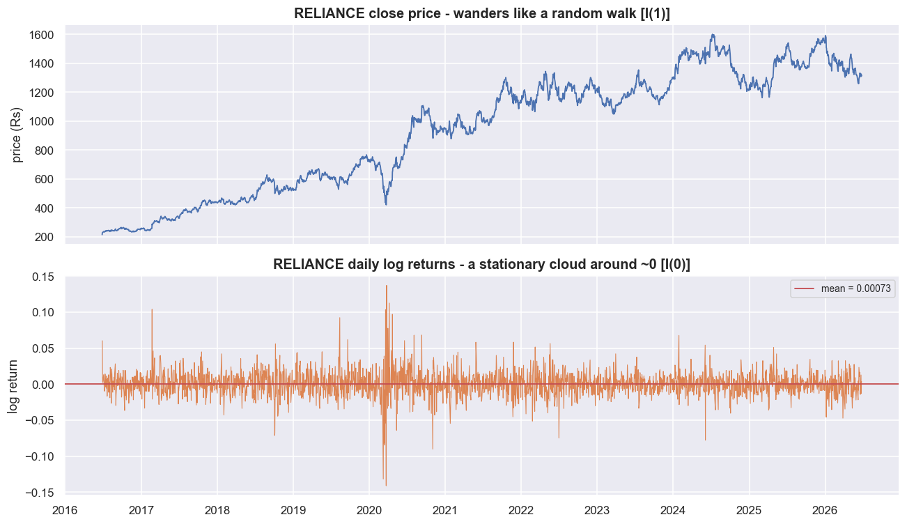
The price chart has no horizontal line you could honestly draw as "fair value." Wherever the price is, it could be twice or half that in a few years. Split the sample in half and the log-price average shifts from 6.272 to 7.156: the centre of the level moves, which is exactly what non-stationarity looks like. The returns chart is the opposite. Its average is pinned near zero in both halves (+0.00124 then +0.00023), and its standard deviation is stable (0.0195 then 0.0141). One caveat we will not hide: returns are stationary in their average, but their volatility comes in clusters - calm stretches and violent ones. That changing volatility is called conditional heteroskedasticity, and it is not the same as non-stationarity; the long-run variance is still finite and stable. It matters a lot for sizing risk, so we flag it now rather than spring it on you later.

The ADF test, read the way it is meant to be read

Eyeballing charts is not evidence. The Augmented Dickey-Fuller (ADF) test is the workhorse. In plain terms, it asks: is this series a random walk, or does it mean-revert? It fits delta y_t = alpha + beta*t + gamma * y_{t-1} + (lagged differences) + e_t and tests H0: gamma = 0 (a unit root - non-stationary) against H1: gamma < 0 (mean-reverting). Two setup choices a professional never leaves on autopilot. First, lag length: the lagged-difference terms mop up short-run memory in the series so the result is valid; too few biases the test, too many wastes power. Use autolag='AIC' to let a standard criterion pick the number for you. Second, the regression form: 'c' includes a constant (the series reverts to a non-zero level), 'ct' adds a straight-line trend, 'n' has neither. And the part most people skip entirely: the test is one-sided and its statistic is negative. The p-value here is the chance, if the series really were a random walk, of seeing a result at least this strong; small means evidence of mean reversion (and, from the primer above, it is not the probability that the random-walk story is true). But do not just compare the p-value to 0.05 and stop. Compare the statistic to the critical values. The more negative the statistic, the stronger the evidence against a unit root.

Copy

# ADF statistic vs critical values, as a chart: more-negative = more evidence against unit root
labels = [f'{STOCK}\nlog price', f'{STOCK}\nlog returns']
stats  = [r_logp['stat'], r_ret['stat']]
colors = [C['red'] if not d['reject5'] else C['green'] for d in (r_logp, r_ret)]
crit   = r_ret['crit']   # same critical values (regression='c')

fig, ax = plt.subplots(figsize=(9.5, 5))
bars = ax.bar(labels, stats, color=colors, width=0.5, edgecolor='white', zorder=3)
for lvl, ls in [('1%', '-'), ('5%', '--'), ('10%', ':')]:
    ax.axhline(crit[lvl], color=C['amber'], lw=1.5, ls=ls, zorder=2,
               label=f'{lvl} critical = {crit[lvl]:.2f}')
ax.axhline(0, color=C['grey'], lw=1)
for b, s in zip(bars, stats):
    ax.text(b.get_x()+b.get_width()/2, s + (0.4 if s < 0 else -0.8), f'{s:.2f}',
            ha='center', va='bottom' if s < 0 else 'top', fontweight='bold')
ax.set_title('ADF statistic vs critical values (regression="c")\nbelow the dashed line = reject unit root = stationary')
ax.set_ylabel('ADF statistic (more negative = more stationary)')
ax.legend(fontsize=9, loc='lower left')
plt.tight_layout(); plt.show()
print("The price bar floats above all three critical lines (a unit root); the returns bar")
print("plunges far below them (decisively stationary). This is the whole notebook in one chart.")

Live output

The price bar floats above all three critical lines (a unit root); the returns bar
plunges far below them (decisively stationary). This is the whole notebook in one chart.

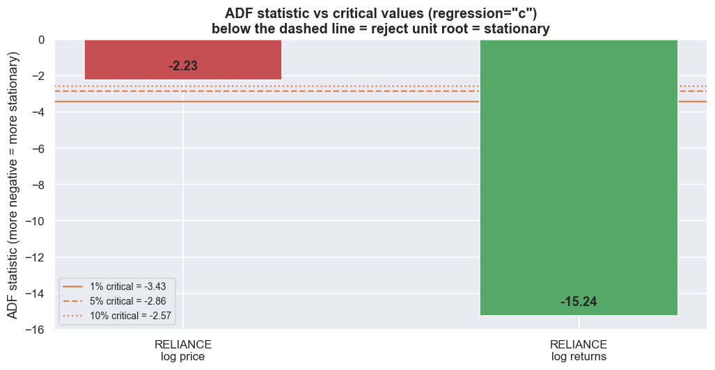
Read it out loud. For RELIANCE's log price, the statistic is -2.234. That sits above (less negative than) even the 10% critical value of -2.567, so we fail to reject the unit root. For its log returns the statistic is -15.241, far below the 1% critical value of -3.433, so we reject decisively. That is the I(1)-price / I(0)-return result, on real data, with the test read correctly. The p-values (0.194 versus 0.000) tell the same story. But the statistic-versus-critical-value reading is the one that holds up on a borderline series.

Now the discipline most people skip: does the verdict survive different setups? Re-run the price test across the choices. The 'c' form with AIC gives -2.234, 'ct' gives -1.997 (and its critical value tightens to -3.412), and the no-constant 'n' form gives a positive +1.825. Every one says "do not reject," so the non-stationary verdict for this price holds up here. But notice how much the statistic moved, and that the 'n' form flipped its sign completely. This kind of agreement is the exception. For the borderline, slow-reverting spreads that stat-arb actually finds, the choice of setup routinely flips the answer - and it is tempting to keep the one that tells you what you want.

The ADF test has a well-known weakness: it under-rejects, meaning it often fails to flag a series that really is mean-reverting. So it is worth running a second test built the other way round. The KPSS test starts from H0: stationary, so rejecting it is evidence for a unit root. For RELIANCE's log price the KPSS statistic is 7.216, far past the 1% critical value of 0.739 - it rejects stationarity. For the returns it is 0.317, below the 5% value of 0.463 - it fails to reject. The two tests now agree from opposite directions, which is the strongest verdict you can get.

One number on the line: the Hurst exponent

ADF and KPSS hand you a yes/no. The Hurst exponent H gives you something richer: a position on a line and a sense of how strong the behaviour is. You estimate it from how the typical size of a move grows as you look over longer and longer gaps: measure the root-mean-square change over a gap of k steps and fit rms(k) ~ k^H on a log-log scale. Then H ~ 0.5 means the series spreads out like a random walk; H < 0.5 means it is mean-reverting (the shape of a tradeable spread); H > 0.5 means it trends and keeps going. Check the estimator first on series whose answer we already know: the synthetic random walk returns 0.502, the AR(1) returns 0.049, white noise -0.004, and a pure drift-plus-trend 0.992. The estimator works. Two cautions, though. Hurst is an estimate, and on finite samples it can come out unstable or even slightly outside the textbook [0, 1] range - white noise here lands at -0.004, a hair below zero, which is sampling noise, not a real negative Hurst. And the value depends on the method (rescaled-range, variance-of-differences, and so on) and on the sample length, so read it as one piece of evidence, never a verdict on its own.

Copy

# Hurst across real NSE log-price series, with synthetic anchors for reference
hnames = ['RELIANCE','TCS','HDFCBANK','ICICIBANK','SBIN','INFY','ITC','HINDUNILVR',
          'MARUTI','SUNPHARMA','TATASTEEL','LT','BHARTIARTL','TITAN']
hvals = {}
for s in hnames:
    try:
        hvals[s] = hurst_vr(np.log(load(s)['close'].dropna().values))
    except Exception as e:
        print('skip', s, e)
hvals['[NIFTY index]']      = hurst_vr(np.log(load('NIFTY', exchange='NSE_INDEX')['close'].dropna().values))
hvals['[synthetic RW]']     = hurst_vr(rw)
hvals['[synthetic AR(1)]']  = hurst_vr(ar)
hs = pd.Series(hvals).sort_values()

fig, ax = plt.subplots(figsize=(11, 6.5))
cols = [C['green'] if v < 0.5 else (C['red'] if v > 0.5 else C['grey']) for v in hs.values]
ax.barh(hs.index, hs.values, color=cols, edgecolor='white', zorder=3)
ax.axvline(0.5, color=C['amber'], lw=2, ls='--', zorder=2, label='H = 0.5  (random walk)')
for y, v in enumerate(hs.values):
    ax.text(v + 0.004, y, f'{v:.2f}', va='center', fontsize=9)
ax.set_title('Hurst exponent on log PRICES: NSE names cluster at ~0.5 (random-walk-like)')
ax.set_xlabel('Hurst exponent  (<0.5 mean-reverting | 0.5 random walk | >0.5 trending)')
ax.legend(loc='lower right'); ax.set_xlim(0, max(0.62, hs.max()+0.06))
plt.tight_layout(); plt.show()

real = hs.drop(['[synthetic RW]','[synthetic AR(1)]'])
print(f"In this window, real NSE log prices have Hurst in [{real.min():.2f}, {real.max():.2f}], "
      f"mean {real.mean():.2f} - i.e. essentially random walks.")
print("No single stock price is a mean-reverter (none sits convincingly below 0.5). That is")
print("exactly why stat-arb builds a SPREAD: the spread, not the price, is where H drops below 0.5.")

Live output

In this window, real NSE log prices have Hurst in [0.46, 0.56], mean 0.50 - i.e. essentially random walks.
No single stock price is a mean-reverter (none sits convincingly below 0.5). That is
exactly why stat-arb builds a SPREAD: the spread, not the price, is where H drops below 0.5.

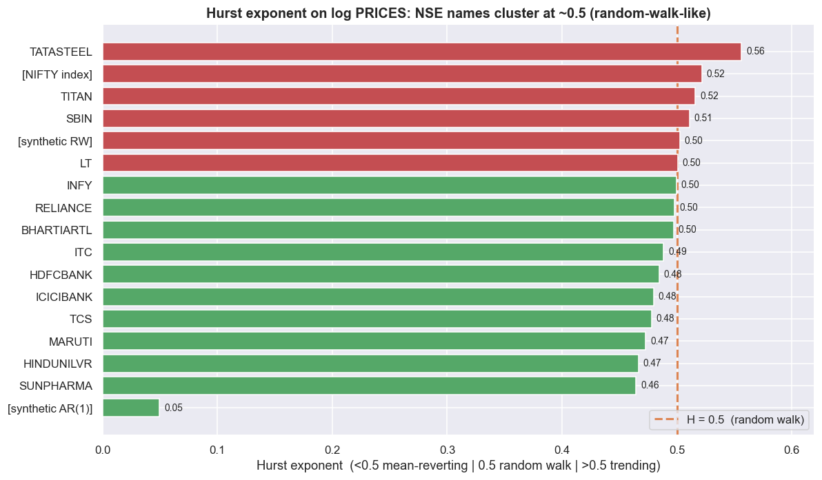
Run it across real NSE log prices and the result is clear: in this window the Hurst exponents land in a tight band of [0.46, 0.56] with a mean of exactly 0.50. No single stock price sits convincingly below 0.5. Not one name is a mean-reverter. The autocorrelation of each series tells the same story. Autocorrelation just measures how much today's value resembles an earlier one. RELIANCE's log price has a lag-1 autocorrelation of 1.000 and one that fades agonisingly slowly - today looks exactly like yesterday, because shocks never leave. Its log returns have a lag-1 autocorrelation of -0.009: essentially no memory from the very first step. There is nothing in the daily return series to exploit directly, and nothing in the price to revert against.

The whole cross-section agrees

One stock could be a fluke. So sweep 24 liquid NSE names. Run ADF (regression='c', autolag='AIC') on each name's log price and its log returns, and collect every verdict in one grid.

Copy

# heatmap of ADF p-values: low (green) = stationary, high (red) = unit root
hm = res[['adf_price','adf_return']].rename(columns={'adf_price':'ADF p\n(log price)',
                                                     'adf_return':'ADF p\n(log return)'})
fig, ax = plt.subplots(figsize=(7, 9))
sns.heatmap(hm, annot=True, fmt='.3f', cmap='RdYlGn_r', vmin=0, vmax=1,
            linewidths=0.5, linecolor='#0d1117', cbar_kws={'label': 'ADF p-value'}, ax=ax)
ax.set_title('ADF p-values across NSE names\nprices = red (unit root) | returns = green (stationary)')
ax.set_ylabel(''); ax.set_xlabel('')
plt.tight_layout(); plt.show()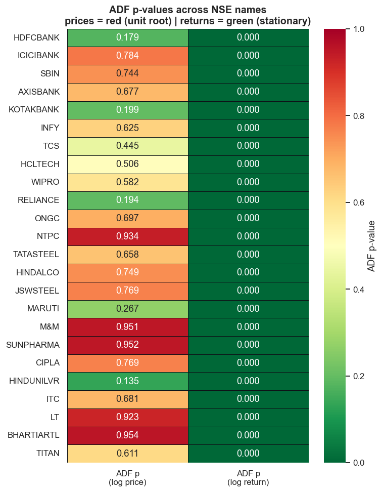

The split is near-total. Every single price fails to reject the unit root - 100% of names, with p-values ranging from 0.13 (HINDUNILVR, the most borderline) up to 0.95 (BHARTIARTL, M&M, SUNPHARMA). Every single return rejects it - 100% of names, with p-values that all round to 0.000. KPSS, built the opposite way, mirrors the verdict exactly: 100% of names reject stationarity on the price, and only 4% - a single name - reject it on returns. There is no ambiguity in this window. Prices are I(1); returns are I(0); and that is why you cannot mean-revert a single stock. The mean-reverting object has to be built - a spread between two co-moving series, engineered so the spread itself is I(0) even though neither leg is. That construction is the subject of the chapters that follow.

Check yourself

Quick self-test before moving on. Try each, then reveal the answer.

1. Why can you sometimes forecast a spread, but almost never a single stock's price level?

A single price is close to a random walk - it has no fixed average to return to, so the level is unforecastable. A spread is built to be stationary: it has a fixed average it keeps returning to, so a move away from that average tends to come back.

2. A daily price series is I(1). What does that mean, and what one operation makes it stationary?

I(1) means you must difference it once to make it stationary. For a price, the log difference (the daily log return) does it: returns are I(0), already stationary.

3. An ADF test on a spread returns p = 0.20. Can you conclude the spread is a random walk?

No. A large p-value means you cannot reject the random-walk null - not that the null is true. Failing to find reversion is not the same as proving there is none, especially with a low-power test on a short sample.

4. A price series shows a Hurst exponent of 0.48. Is that proof it mean-reverts?

No. 0.48 is barely below 0.5 and well inside finite-sample noise. Hurst is one sliding-scale clue, not a standalone proof - confirm with ADF and KPSS, and out of sample.

Where this breaks

Stationarity testing feels like a clean measurement, but it is not. Each honest caveat below comes back to bite real research.

ADF has low power near a unit root. "Power" here means the test's ability to catch mean reversion when it is genuinely there. This is not a footnote - it is the single most important caveat in applied cointegration work. A truly stationary AR(1) with phi close to 1 (slow mean reversion) is one the ADF test routinely cannot tell apart from a random walk in a few thousand observations. Make it concrete: simulate series that are stationary by construction, then ask how often ADF correctly rejects.

Copy

# demonstration: ADF's low power against a near-unit-root (but truly STATIONARY) AR(1)
rngp = np.random.default_rng(20)
def adf_rejects(phi_, npts=1500, reps=300):
    hits = 0
    for _ in range(reps):
        e = rngp.standard_normal(npts); y = np.zeros(npts)
        for t in range(1, npts):
            y[t] = phi_*y[t-1] + e[t]           # stationary for |phi|<1, so TRUTH = stationary
        if adfuller(y, regression='c', autolag='AIC')[1] < 0.05:
            hits += 1
    return hits/reps

phis = [0.80, 0.90, 0.95, 0.98, 0.99]
power = {p: adf_rejects(p) for p in phis}
fig, ax = plt.subplots(figsize=(9.5, 4.6))
ax.bar([str(p) for p in phis], [power[p] for p in phis], color=C['purple'], edgecolor='white', zorder=3)
ax.axhline(1.0, color=C['green'], ls=':', lw=1.2, label='ideal: always reject (series IS stationary)')
for i, p in enumerate(phis):
    ax.text(i, power[p]+0.02, f'{power[p]:.0%}', ha='center', fontweight='bold')
ax.set_title('ADF power collapses as phi -> 1 (all series here are TRULY stationary)')
ax.set_xlabel('AR(1) coefficient phi (closer to 1 = slower mean reversion)')
ax.set_ylabel('fraction ADF correctly rejects @5%'); ax.set_ylim(0, 1.12); ax.legend(fontsize=9)
plt.tight_layout(); plt.show()
print("Every one of these AR(1) series is stationary by construction, yet power collapses as phi -> 1:")
print(f"at phi=0.99 ADF correctly rejects only ~{power[0.99]:.0%} of the time (vs ~{power[0.80]:.0%} at phi=0.80).")
print("'Failed to reject' often means 'too little data', not 'unit root' - the single most important")
print("caveat in applied cointegration work.")

Live output

Every one of these AR(1) series is stationary by construction, yet power collapses as phi -> 1:
at phi=0.99 ADF correctly rejects only ~61% of the time (vs ~100% at phi=0.80).
'Failed to reject' often means 'too little data', not 'unit root' - the single most important
caveat in applied cointegration work.

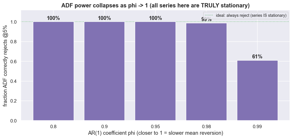
At phi = 0.80 the test correctly rejects ~100% of the time. At phi = 0.99 - still perfectly stationary - it rejects only ~61%. Roughly two times in five it calls a unit root that is not there. The brutal consequence: "ADF didn't reject" is not proof of a unit root. Very often it is just weak data. And the spreads stat-arb actually finds sit right in this dangerous zone - slow mean-reverters with phi near 1, where the tests are least reliable and where the half-life (how long, on average, a deviation takes to shrink by half) is long enough that costs eat the edge before reversion arrives.

Other failure modes pile on. Setup sensitivity: 'c' versus 'ct' versus 'n', and the lag length, can flip a borderline verdict - so decide the setup before you look, never after. Structural breaks: every test here assumes one fixed regime. A pair that was stationary for three years and broke after a merger or an index reshuffle will still test "stationary" on the combined sample while being untradeable now. Stationarity over the whole window says nothing about stationarity going forward. Small samples and fat tails: the critical values are only exact for very long samples, daily equity returns have heavy tails and clustered volatility, and the KPSS p-value is read off a small lookup table - so treat every p-value as a rough guide, not a precise number. And the deepest caveat of all: stationary is necessary, not sufficient. Even a perfect I(0) spread is not yet a strategy. It still has to revert faster than costs pile up, survive out-of-sample (on fresh data you never used to build it), and be tradable on both legs in the Indian market - the gap this whole series exists to expose.