Building the Historical Database

Every other chapter in this course opens a price panel in a fraction of a second and goes straight to the statistics. That speed hides something. Somebody had to pull ten years of daily bars for fifty names plus the index, once, and store them in a local database so nobody ever has to ask the broker for them again. This chapter is that somebody. It is the unglamorous plumbing under the whole module: where the data comes from, how it is stored, and - the part most tutorials skip - how you prove the cache is actually complete before you trust a single spread built on top of it. Get this wrong and every elegant cointegration test downstream is computing beautiful statistics on quietly broken data.

Download once, read fast

The easiest way to waste a research afternoon is to re-download history on every run. A single ten-year daily series is only a few hundred kilobytes over the wire - tiny. But fifty of them, pulled again and again while you iterate on ideas, add up to thousands of network round-trips you never needed. And the API is rate-limited, so it will eventually push back.

The fix is a local cache. You pay the download cost exactly once, with source="api". After that, every source="db" read is a local scan with no network in the path at all. OpenAlgo's store is a DuckDB file on disk. The two modes look like this: the slow, networked first run, and the instant steady state on every run after it.

The fifty names and the index

The universe is the fifty current Nifty 50 stocks plus the NIFTY index itself. We group them by sector, so that same-sector pairs - the natural hunting ground for a mean-reverting spread - sit next to each other. In this build that is fifty stocks across fourteen sectors: five private banks, the NBFC and insurance block, IT, metals, energy, autos, pharma, FMCG, materials, infra and the rest. The stocks live on exchange NSE. The index lives on its own exchange, NSE_INDEX. That matters: you fetch it with a different argument, and later it becomes your trusted trading-day calendar.

One warning you should hear now, and again at the end: this is today's index membership, cached backwards. That single fact is the most flattering bias in the whole course, and we come back to it hard in the final section.

db vs api, measured

An expert does not take "the cache is faster" on faith. Time the same call both ways on one liquid name, a few repeats each, and report the measured ratio. The api path crosses the network to the broker and re-packages the response. The db path is a local DuckDB query. The exact numbers depend on your machine and the broker's mood, but the shape never changes.

Copy

import time
def time_call(source, n=4):
    ts = []
    for _ in range(n):
        t0 = time.perf_counter()
        client.history(symbol='KOTAKBANK', exchange='NSE', interval='D',
                       start_date=START, end_date=END, source=source)
        ts.append(time.perf_counter() - t0)
    return np.array(ts)

db_t  = time_call('db')
api_t = time_call('api')
db_med, api_med = np.median(db_t), np.median(api_t)
speedup = api_med / db_med
print(f'source="db"  median {db_med*1000:7.1f} ms   (min {db_t.min()*1000:.1f} ms)')
print(f'source="api" median {api_med*1000:7.1f} ms   (min {api_t.min()*1000:.1f} ms)')
print(f'\n--> in this run, db is {speedup:.1f}x faster than api on a 10-year daily series')

tdf = pd.DataFrame({'source': ['db (cache)', 'api (broker)'],
                    'ms': [db_med*1000, api_med*1000]})
fig, ax = plt.subplots(figsize=(8, 3.2))
sns.barplot(data=tdf, x='ms', y='source', hue='source',
            palette=[C['blue'], C['amber']], legend=False, ax=ax)
ax.set_title(f'One 10-year daily read: db vs api  ({speedup:.1f}x)'); ax.set_xlabel('milliseconds (median of 4)')
ax.set_ylabel('')
for i, v in enumerate([db_med*1000, api_med*1000]):
    ax.text(v, i, f'  {v:.0f} ms', va='center', color=C['grey'])
plt.tight_layout(); plt.show()

Live output

source="db"  median    54.7 ms   (min 44.0 ms)
source="api" median   346.0 ms   (min 173.3 ms)

--> in this run, db is 6.3x faster than api on a 10-year daily series

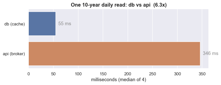
In this data window the db read came back in a median 54.7 ms, against the api path's 346.0 ms - the cache is 6.3x faster on a single ten-year daily series. Multiply that by fifty names over a session of dozens of re-runs. The gap stops being a convenience and becomes the difference between an idea you can keep iterating on and one you abandon out of boredom.

Inside the cache: the market_data table

OpenAlgo stores every bar in a DuckDB table called market_data, one row per (symbol, exchange, interval, timestamp). The timestamp is a Unix epoch in seconds: integer keys are small, sort fast, and never trip over a timezone. A second table, data_catalog, summarises each series - its first timestamp, last timestamp, record count and last download time - so you can check coverage without scanning the bars themselves. Writing a downloaded OHLCV frame into this schema is a tidy transform: cast the index to epoch seconds, force volume and open interest to integers, then insert. Reading the catalog back out is a single GROUP BY symbol that any verification routine can trust.

Verifying coverage: rows, spans, and gaps

A download that ran is not the same as a download that succeeded. Before trusting fifty series for research, you check every one - row count, first date, last date - and flag anything short or missing. Importantly, this check uses source="db" only: a pure local scan, no more downloads. The first view is simply how many daily bars each name carries.

Copy

order = cov.sort_values('rows').index.tolist()
fig, ax = plt.subplots(figsize=(11, 12))
sns.barplot(data=cov.reset_index(), y='symbol', x='rows', hue='sector',
            order=order, dodge=False, palette='tab20', ax=ax)
ax.axvline(med, color=C['grey'], ls='--', lw=1)
ax.text(med, len(order)-1, f'  median {med}', color=C['grey'], va='top', fontsize=9)
ax.set_title('Daily bars cached per symbol (source="db")'); ax.set_xlabel('rows'); ax.set_ylabel('')
ax.legend(title='sector', bbox_to_anchor=(1.01, 1), loc='upper left', fontsize=7, ncol=1)
plt.tight_layout(); plt.show()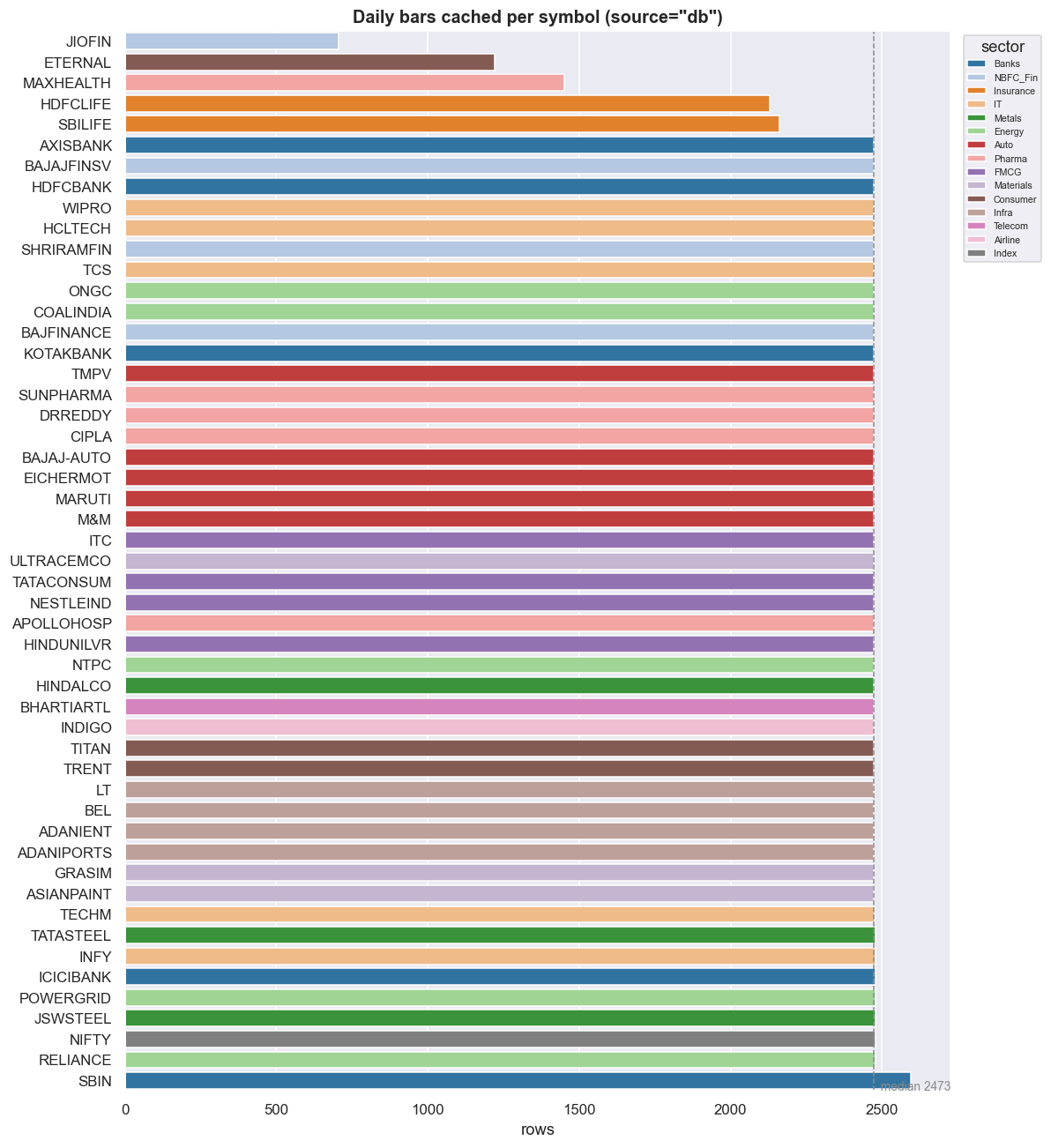

A healthy daily cache is a flat block of bars against the same ceiling, with a handful of short stubs. In this window the index calendar prints 2,477 sessions, and the full-history names sit right up against it. The stubs - JIOFIN, ETERNAL, TMPV, SHRIRAMFIN - are genuinely younger series: recent listings or symbol renames, not data errors. You confirm that by looking at when each series starts, not just how many rows it has.

Copy

import matplotlib.dates as mdates
ordsp = cov.sort_values('first', ascending=False).index.tolist()
fig, ax = plt.subplots(figsize=(11, 12))
common_last = pd.to_datetime(cov['last']).max()
for i, s in enumerate(ordsp):
    a, b = pd.to_datetime(cov.loc[s, 'first']), pd.to_datetime(cov.loc[s, 'last'])
    short = cov.loc[s, 'flag'] == 'SHORT'
    stale = (common_last - b).days > 7
    col = C['red'] if stale else (C['amber'] if short else C['blue'])
    ax.plot([a, b], [i, i], lw=4, color=col, solid_capstyle='round')
ax.set_yticks(range(len(ordsp))); ax.set_yticklabels(ordsp, fontsize=7)
ax.set_ylim(-1, len(ordsp))
ax.xaxis.set_major_locator(mdates.YearLocator()); ax.xaxis.set_major_formatter(mdates.DateFormatter('%Y'))
ax.set_title('Cache coverage span per series  (amber = shorter history, blue = full, red = stale)')
plt.tight_layout(); plt.show()
print('all series end on/around:', cov["last"].max(), '| earliest start:', cov["first"].min())

Live output

all series end on/around: 2026-06-25 | earliest start: 2016-01-01

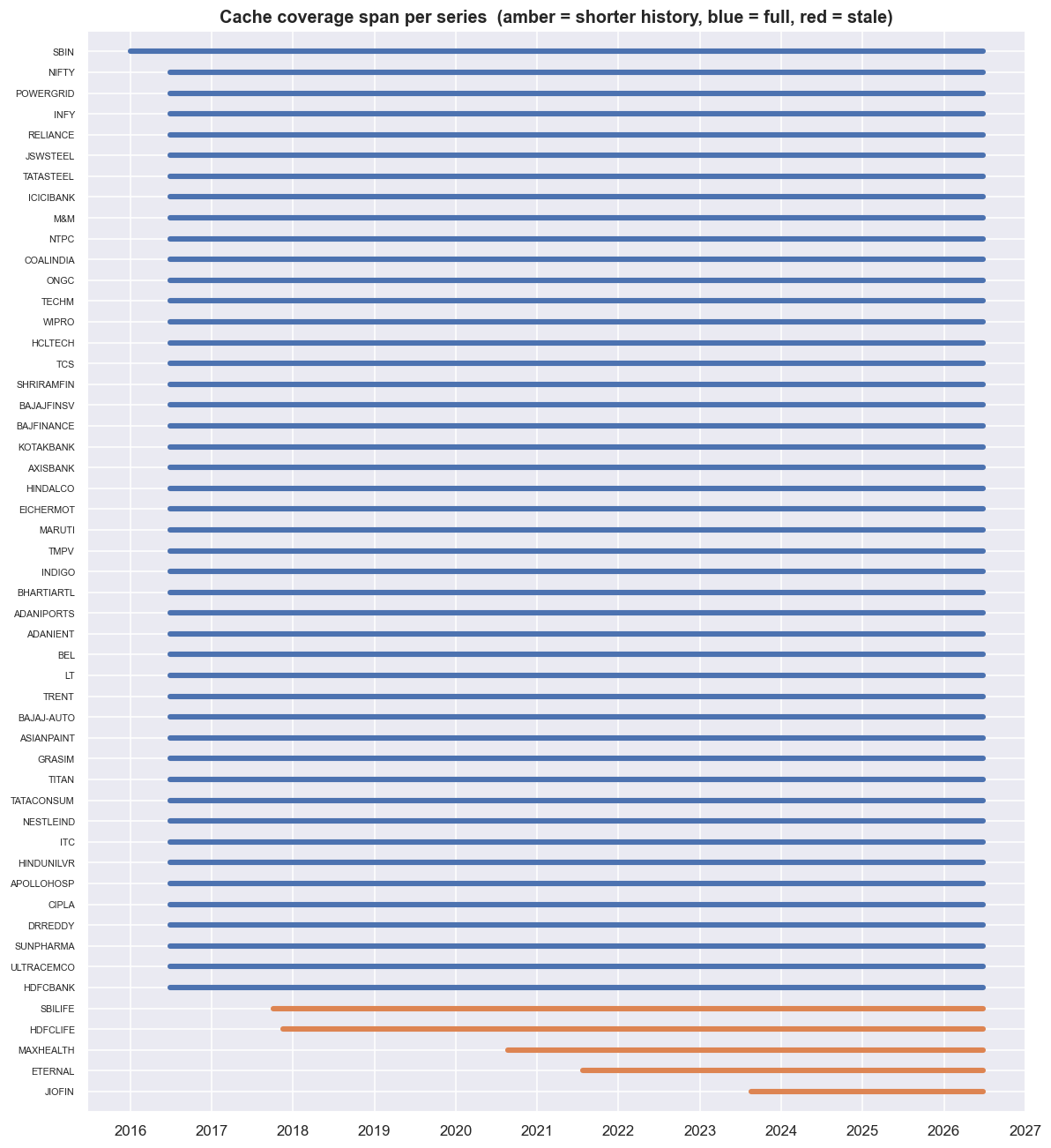
Row counts tell you how many bars. The span view tells you which window they cover. Each bar runs from a series' first cached date to its last. Across this cache the earliest start is 2016-01-01, and every series ends on or around 2026-06-25 - the last common trading day. That lined-up right edge is the thing you are checking for. A series that stopped early would be one nobody topped up. On a two-legged spread that is not a small problem: a stale leg silently freezes one side of the relationship while the other side keeps moving.

But row counts and spans can both look healthy and still hide holes inside the series - a missing Tuesday here, a skipped week there - that quietly corrupt a spread without ever showing up as a short history. To find them you need the exact list of dates the market was actually open. Rather than hardcode a holiday list that goes stale, use the NIFTY index series as the trusted NSE trading-day calendar: by definition, the index prints on every trading day. For each symbol, within its own active window, a gap is any NIFTY session it is missing.

Copy

nifty_sessions = pd.DatetimeIndex(idx_of['NIFTY'])
def internal_gaps(symbol):
    have = pd.DatetimeIndex(idx_of[symbol])
    win = nifty_sessions[(nifty_sessions >= have.min()) & (nifty_sessions <= have.max())]
    return int(len(win.difference(have)))

gaps = pd.Series({s: internal_gaps(s) for s in idx_of if s != 'NIFTY'}).sort_values(ascending=False)
print(f'sessions in the NIFTY calendar (window): {len(nifty_sessions)}')
print(f'symbols with zero internal gaps: {(gaps == 0).sum()} of {len(gaps)}')
print(f'worst-case internal gaps for any single name: {gaps.max()} sessions\n')
print('most gaps (a handful is normal: trading halts, suspensions, calendar edge effects):')
print(gaps.head(10))

top = gaps[gaps > 0].head(15)
if len(top):
    fig, ax = plt.subplots(figsize=(10, 5))
    sns.barplot(x=top.values, y=top.index, hue=top.index, palette='rocket', legend=False, ax=ax)
    ax.set_title('Internal missing sessions vs the NIFTY calendar (top names)')
    ax.set_xlabel('missing sessions'); ax.set_ylabel('')
    plt.tight_layout(); plt.show()
else:
    print('no internal gaps anywhere - a clean cache')

Live output

sessions in the NIFTY calendar (window): 2477
symbols with zero internal gaps: 10 of 50
worst-case internal gaps for any single name: 3 sessions

most gaps (a handful is normal: trading halts, suspensions, calendar edge effects):
HDFCBANK      3
AXISBANK      3
WIPRO         3
KOTAKBANK     3
BAJFINANCE    3
BAJAJFINSV    3
SHRIRAMFIN    3
HINDALCO      3
TCS           3
HCLTECH       3
dtype: int64

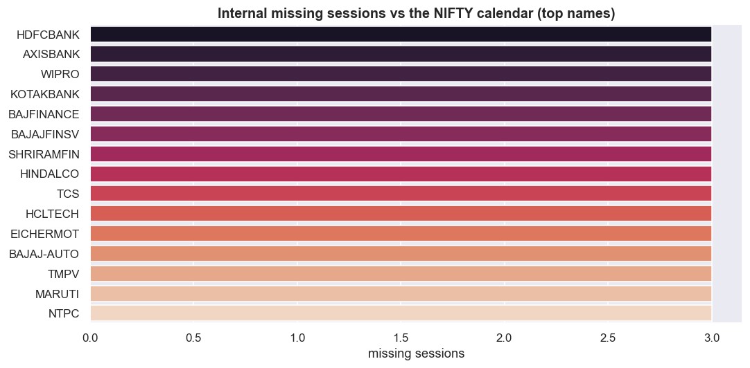
The verdict in this data window: against a 2,477-session calendar, 10 of 50 names are perfectly clean, and the worst single name is missing just 3 sessions. Three. Those are almost certainly real trading halts or suspensions, not corruption - the kind of thing a sane cache lives with. But notice what this check buys you. It is the difference between "the file loaded" and "the file is right." If one name had been missing forty sessions, the row count alone might never have flagged it, and you would have found the hole the hard way: as a fake jump in a spread weeks later.

Keeping it current without re-downloading

Once the cache exists, keeping it current must be cheap. The wrong way is to re-download ten years every morning. The right way is to ask the cache for each symbol's last date, fetch only [last+1 .. today] from the API, then append with de-duplication so an overlapping re-fetch costs nothing.

And because a real download loop hits the API hundreds of times, wrap every fetch in exponential backoff. On a timeout or a too many requests error, wait, then double the wait a few times before giving up. It is ten lines of code, and it is the difference between a download that survives a flaky network and one that dies half-written at symbol thirty.

Where this breaks

This cache is a convenience, not a source of truth. The honest failure modes:

• Rate limits and partial downloads. A fifty-symbol pull is hundreds of API calls, and a mid-run 429 or timeout can leave a series half-written. The retry wrapper helps, but the real guard is the verification pass above. Never assume a bulk download finished - re-check coverage and gaps every time.
• Adjustment is baked in at download time. The bars are whatever the broker served on the day they were fetched - usually adjusted for splits and dividends up to that date. A later corporate action re-adjusts history at the vendor, so an old cached series can quietly disagree with a fresh pull. The cached close is for measuring relationships, not for reconstructing the exact rupee price you could have traded at.
• Vendor gaps and bad prints. Missing sessions, zero-volume days, the odd spike or stale carried-forward price come straight from the upstream feed. Gap detection finds the holes; it does not fix a wrong price. A spread is unforgiving of a single bad bar on one leg.
• Point-in-time and survivorship. This is today's Nifty 50, cached backwards. Names that were dropped, merged or delisted are simply absent, and recent renames - ETERNAL, TMPV, JIOFIN, SHRIRAMFIN - have broken histories. A backtest on this universe is biased toward survivors. A true point-in-time database that keeps the delisted names is out of scope here, but it is the limitation that most flatters every result downstream, and you should never forget it is there.

With the database built, verified and kept current, the rest of the course simply reads it with source="db". The next chapter assembles the clean research panel from this cache, and spells out the trading-price-versus-adjusted-price caveats in full.