Cross-Sectional, Factor-Neutral Stat Arb

Every strategy so far has traded one relationship at a time - a single pair, a Kalman-tracked pair, or a Johansen basket. They all hit the same ceiling. One spread can only hold so much money. And the day the relationship breaks, you are left with a hedge ratio - the recipe for how much of stock B you trade against stock A - that has simply stopped working. This chapter builds the version of statistical arbitrage with no such ceiling. It runs across a whole universe of stocks at once, and it is market-neutral by design - built so that broad market moves cancel out. This is the workhorse of every equity market-neutral desk, and the most scalable idea in the course. It is also the cleanest example of the course's main lesson: a statistical relationship existing is not the same thing as a tradeable edge existing. The signal here is real, clean, and genuinely market-neutral before costs. But the book trades so much, so often, that realistic NSE costs do more than dent the edge - they flip its sign from profit to loss.

Strip the market, keep the wiggle

The whole idea fits in one sentence. Most of a stock's daily move is just the market (and its sector) moving up or down. Strip that shared move out, and what is left tends to over-react and then snap back. That leftover is called the residual - the part of the day that is unique to the stock, not explained by the market. The tool that separates the two is a simple regression. Take one stock and fit a line between its daily return and the NIFTY return. The slope of that line is the stock's beta - how strongly it moves with the market. The scatter of points around the line is the residual.

Copy

import statsmodels.api as sm
demo = 'AXISBANK'
d = pd.DataFrame({'mkt': mret, 'stk': rets[demo]}).dropna()
ols = sm.OLS(d['stk'], sm.add_constant(d['mkt'])).fit()
b_full, r2 = ols.params['mkt'], ols.rsquared
d['resid'] = ols.resid

fig, (axL, axR) = plt.subplots(1, 2, figsize=(13, 5))
sns.regplot(data=d, x='mkt', y='stk', ax=axL, scatter_kws=dict(s=8, alpha=0.25, color=C['blue']),
            line_kws=dict(color=C['amber'], lw=2.2))
axL.set_title(f'{demo} daily return vs NIFTY  (beta={b_full:.2f}, R^2={r2:.2f})')
axL.set_xlabel('NIFTY daily log return'); axL.set_ylabel(f'{demo} daily log return')
axL.axhline(0, color=C['grey'], lw=.6); axL.axvline(0, color=C['grey'], lw=.6)

sns.histplot(d['resid'], bins=80, color=C['green'], ax=axR, stat='density')
axR.set_title(f'{demo} RESIDUAL (return minus beta . NIFTY)')
axR.set_xlabel('residual daily return'); axR.axvline(0, color=C['red'], ls='--', lw=1.2)
plt.tight_layout(); plt.show()

print(f'{demo}: market explains R^2={r2*100:.0f}% of its daily variance; '
      f'the residual std is {d["resid"].std()*100:.2f}% vs raw {d["stk"].std()*100:.2f}% per day.')
print('A single-stock position is mostly a market position. The residual is the small part we can isolate.')

Live output

AXISBANK: market explains R^2=51% of its daily variance; the residual std is 1.48% vs raw 2.11% per day.
A single-stock position is mostly a market position. The residual is the small part we can isolate.

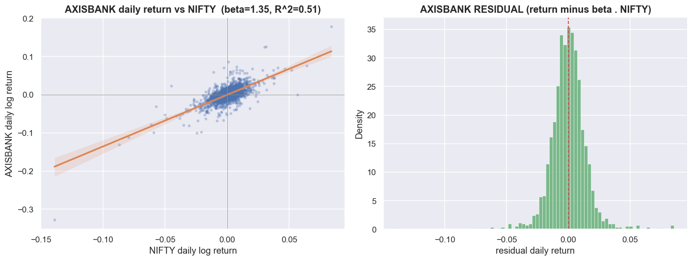
For AXISBANK, the market alone explains 51% of its daily variance (that is the R-squared). The residual moves about 1.48% per day, against a raw 2.11% for the stock itself. Read this the right way round. When you simply buy a stock, you are mostly buying the market, with a small stock-specific extra riding on top. A market-neutral book is only allowed to bet on that small extra. Across the full 50-name universe, removing the market takes out a median 31% of each stock's daily variance. Also removing the average move of its sector lifts that to a median 61%. So roughly two-thirds of a typical stock's daily move is market plus sector. The residual book trades only the remaining third.

Two honesty rules are built in from the start. First, the beta is a 120-day rolling estimate. The beta on any day uses only the returns up to that day, never future data. Second, the sector adjustment subtracts the same-day average move of the sector. So if two banks both jump on a banking-policy headline, that shared jump does not create a fake signal between them. One timing caveat: this same-day sector average is only known at the close, so a signal built from it can be acted on no earlier than the next bar. That is fine for end-of-day research, but treating it as tradable before the close would be look-ahead. The notebook's own note says it well: "optionally remove sector" is not really optional. Removing the sector is where most of the clean edge lives.

From residual to a market-neutral book

The residual is the raw material. The signal is built from it in two steps. First, take each stock's residual added up over the last k days, and flip its sign. Second, subtract the average signal across all stocks - this step is called demeaning. A stock whose residual has fallen hard over the last couple of days gets a high signal and becomes a buy candidate. One whose residual has run up gets a low signal and becomes a short. Demeaning is what makes the book dollar-neutral - equal money long and short - because once you subtract the average, the longs and shorts have to balance.

Turning that signal into an actual book is three lines of arithmetic. Rank the names each day. Demean the ranks so longs and shorts offset. Then scale so the gross book - the total size you actually trade, long plus short - equals 1, which works out to about 0.5 long and 0.5 short. The weights sum to zero, and the residuals already had their beta stripped out, so the book is dollar-neutral and roughly market-neutral. The book's actual beta in this window comes out at a mean of +0.006 with a standard deviation of 0.058 - about as close to zero as a real book ever gets. On a typical recent day the longs were the residual losers (BHARTIARTL, BEL, BAJAJ-AUTO, SUNPHARMA, ONGC, ETERNAL) and the shorts were the residual winners (INDIGO, M&M, RELIANCE, MAXHEALTH, TRENT, ADANIENT). None of these is a bet on the market going up or down. Each one is a bet that the stock's own residual stretched too far and will snap back.

The edge is real - the decile test says so

An equity curve can make a weak strategy look good, so before plotting any profit, ask a cleaner question. Does the signal actually sort future returns in the right order? To check, line up every stock each day and split them into ten equal buckets by signal - these buckets are called deciles. Decile 0 is the strongest short, decile 9 the strongest buy. Then average each bucket's next-day residual return.

Copy

fret = residSN.shift(-1)                                   # next-day residual return
S = build_signal(residSN, K).stack(); F = fret.stack()
dd = pd.DataFrame({'sig': S, 'fwd': F}).dropna()
dd['dec'] = dd.groupby(level=0)['sig'].transform(
    lambda x: pd.qcut(x.rank(method='first'), 10, labels=False))
dec = dd.groupby('dec')['fwd'].mean() * 1e4                # bps/day

fig, ax = plt.subplots(figsize=(11, 5))
sns.barplot(x=dec.index.astype(int), y=dec.values,
            hue=dec.index.astype(int), palette='RdYlGn', legend=False, ax=ax)
ax.axhline(0, color=C['grey'], lw=.9)
ax.set_title(f'Mean NEXT-DAY residual return by signal decile (k={K})  '
             f'-- 0 = short candidates, 9 = long candidates')
ax.set_xlabel('signal decile (low -> high)'); ax.set_ylabel('mean forward residual (bps/day)')
plt.tight_layout(); plt.show()
spread = dec.iloc[-1] - dec.iloc[0]
print(f'top-minus-bottom decile spread: {spread:+.2f} bps/day gross.')
print('Broadly monotonic with a noisy extreme decile -- the honest signature of a real but THIN edge,')
print('not the clean staircase a curve-fit would draw.')

Live output

top-minus-bottom decile spread: +3.89 bps/day gross.
Broadly monotonic with a noisy extreme decile -- the honest signature of a real but THIN edge,
not the clean staircase a curve-fit would draw.

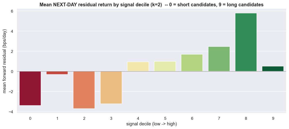
The buckets climb, broadly, from left to right. The gap between the top bucket and the bottom one is +3.89 basis points per day before costs (a basis point is one-hundredth of a percent). Notice the shape, which the notebook is honest about. It mostly rises bucket by bucket, but the extreme bucket is noisy. It is not the perfect, clean staircase a curve-fitted result would draw. That noise is the honest signature of a real but thin edge.

The factor model is the step that strips out the market and the sector - the two big shared forces, or "factors", that move many stocks together. It genuinely matters here, and is not wasted effort. Removing only the market gives a gross Sharpe of 0.51 - the Sharpe ratio is return divided by risk, where higher is better and below about 1 after costs is weak. Also removing the sector's average move lifts the gross Sharpe to 1.34. The shared movement inside a sector was adding noise to the ranking, and removing it roughly doubles the clean edge. A gross Sharpe a little above 1.3 on a truly market-neutral book is exactly the steady, low-volatility profile a desk is built to harvest. So we have a real signal that sorts returns, and a real modelling step that nearly doubles it. Everything up to here is the good news.

Then you try to harvest it

Here is the whole argument of the chapter on one chart. The gross curve is that clean residual-reversion edge grinding steadily upward, with only a shallow drawdown. Then we subtract realistic NSE trading costs.

Copy

bt_cnc, _ = backtest(residSN, K, COST_CNC)
gE, nM, nC = eqc(bt['gross']), eqc(bt['net']), eqc(bt_cnc['net'])
pM, pC = perf(bt['net']), perf(bt_cnc['net'])

fig, ax = plt.subplots(figsize=(12, 5.6))
ax.plot(gE.index, gE.values, color=C['green'], lw=2.2,
        label=f'GROSS              Sharpe {g["sharpe"]:.2f}   {g["total"]*100:+.0f}%')
ax.plot(nM.index, nM.values, color=C['amber'], lw=2.0,
        label=f'NET (MIS, intraday)  Sharpe {pM["sharpe"]:.2f}   {pM["total"]*100:+.0f}%')
ax.plot(nC.index, nC.values, color=C['red'],   lw=2.0,
        label=f'NET (CNC, overnight) Sharpe {pC["sharpe"]:.2f}   {pC["total"]*100:+.0f}%')
ax.axhline(1, color=C['grey'], lw=.8, ls=':')
ax.set_title(f'Cross-sectional residual reversion (k={K}): gross is real, net is the problem')
ax.set_ylabel('growth of Rs 1 (gross book = 1)'); ax.legend(loc='upper left', fontsize=10)
plt.tight_layout(); plt.show()
print('Same signal, same days. The only thing that changed is whether we paid to trade it.')

Live output

Same signal, same days. The only thing that changed is whether we paid to trade it.

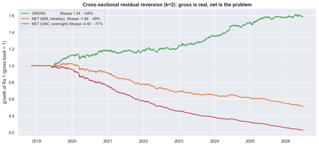
It is the same signal, on the same days. The only thing that changes is whether you pay to trade it. Gross means before trading costs; net means after. The gross Sharpe of 1.34 becomes a net Sharpe of -1.99 once you charge intraday (MIS) costs. Under overnight (CNC) costs, which carry the heavier delivery tax, the curve does not just flatten - it falls off a cliff. This is not a small haircut. In the pairs chapter, costs turned a gross 0.90 into a net 0.77 - just a trim, because a plus-or-minus-two-sigma rule trades rarely. Here, costs take a positive 1.34 and hand back a negative 1.99. The edge is not reduced. Its sign is reversed. A strategy that made money before costs reliably loses money after them.

Turnover is the whole story

Why does a 1.34-Sharpe signal die this badly when a pairs trade survived? One number explains it: turnover - how much of the book you trade over a period. This book trades close to its entire gross value every single day, which adds up to roughly 235 times a year. The signal works on a one-to-three-day horizon and flips constantly, so almost the whole book is replaced daily. High turnover means costs pile up fast.

Copy

fig, (axT, axD) = plt.subplots(2, 1, figsize=(12, 7), sharex=True,
                               gridspec_kw=dict(height_ratios=[1, 1]))
roll_turn = bt['turn'].rolling(21).mean()
axT.plot(roll_turn.index, roll_turn.values, color=C['blue'], lw=1.5)
axT.axhline(bt['turn'].mean(), color=C['red'], ls='--', lw=1.2,
            label=f'mean {bt["turn"].mean():.2f}/day')
axT.set_title('One-way turnover (21-day mean) -- close to the whole book, every day')
axT.set_ylabel('turnover / day'); axT.legend(loc='upper right')

daily_edge = bt['gross'].rolling(21).mean() * 1e4
daily_cost = (bt['turn'] * COST_MIS).rolling(21).mean() * 1e4
axD.plot(daily_edge.index, daily_edge.values, color=C['green'], lw=1.6, label='gross edge (bps/day)')
axD.plot(daily_cost.index, daily_cost.values, color=C['amber'], lw=1.6, label='MIS cost drag (bps/day)')
axD.fill_between(daily_edge.index, daily_edge.values, daily_cost.values,
                 where=(daily_cost.values > daily_edge.values), color=C['red'], alpha=0.18)
axD.axhline(0, color=C['grey'], lw=.8)
axD.set_title('Gross edge vs cost drag (21-day mean) -- red = costs exceed the edge')
axD.set_ylabel('bps / day'); axD.legend(loc='upper right'); axD.set_xlabel('')
plt.tight_layout(); plt.show()
print(f'annualised one-way turnover ~ {bt["turn"].mean()*252:.0f}x the gross book.')
print(f'gross ~ {bt["gross"].mean()*1e4:.2f} bps/day vs MIS cost ~ {(bt["turn"]*COST_MIS).mean()*1e4:.2f} bps/day.')

Live output

annualised one-way turnover ~ 235x the gross book.
gross ~ 2.48 bps/day vs MIS cost ~ 6.45 bps/day.

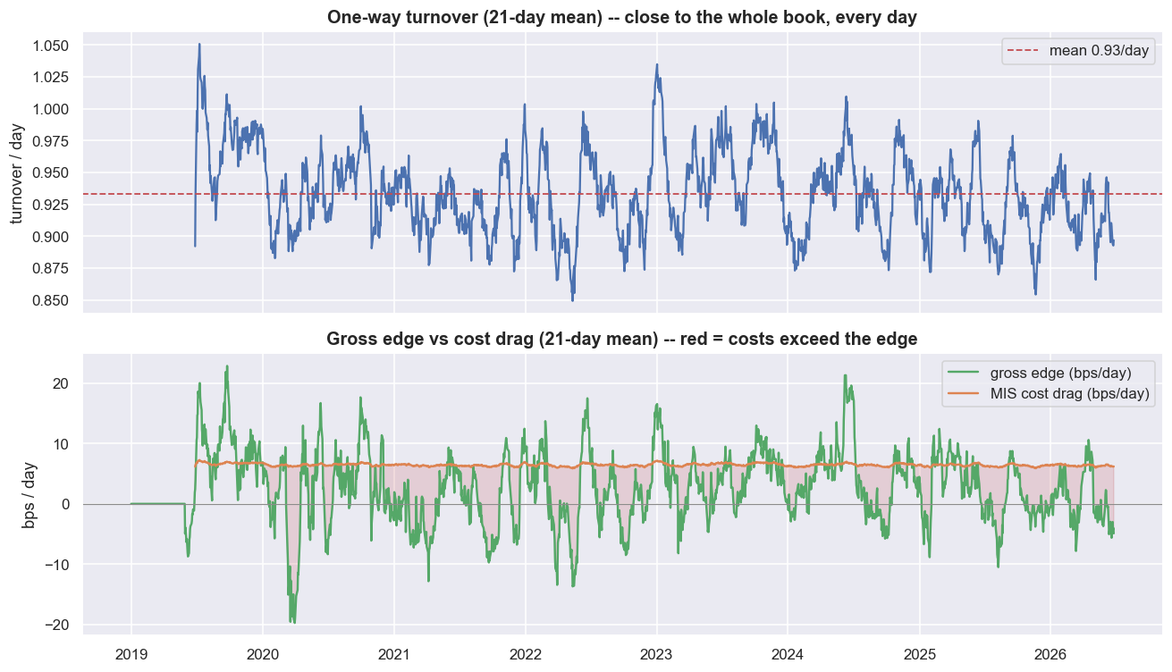
Now do the arithmetic a desk does. The gross edge is about 2.48 bps per day. The MIS cost, at this much turnover, is about 6.45 bps per day. You are paying roughly two and a half times your edge just to capture it. The red shaded region - where cost sits above edge - covers most of the chart.

The one lever that genuinely helps is trading less often. Stretching the lookback k from 1 to 20 days slows the signal and cuts turnover from 1.34x to 0.31x per day. The net Sharpe then climbs from -3.83 at k=1 toward -0.16 at k=15. It climbs, but it never crosses zero. Even at the slowest, stalest setting, the residual edge is too thin to clear the cost. You cannot out-think turnover with a better factor model, and you cannot out-wait it with a longer holding period. The clearest way to see the verdict is to flip the question around and ask how cheap you would need to be.

Copy

b0, _ = backtest(residSN, K, 0.0)            # gross once; cost is linear in cost_side
gross_mu, turn_mu = b0['gross'].mean(), b0['turn'].mean()
breakeven_bps = gross_mu / turn_mu * 1e4
cps = np.linspace(0, 14, 80)                 # per-side cost in bps
net_ann = (gross_mu - (cps/1e4) * turn_mu) * 252 * 100   # annualised net return, %

fig, ax = plt.subplots(figsize=(11.5, 5.2))
ax.plot(cps, net_ann, color=C['purple'], lw=2.4)
ax.axhline(0, color=C['grey'], lw=1.0)
ax.fill_between(cps, net_ann, 0, where=(net_ann > 0), color=C['green'], alpha=.18)
ax.fill_between(cps, net_ann, 0, where=(net_ann < 0), color=C['red'],   alpha=.15)
ax.axvline(breakeven_bps, color=C['grey'], ls=':', lw=1.4)
ax.text(breakeven_bps, ax.get_ylim()[1]*0.9, f'  breakeven {breakeven_bps:.1f} bps/side', fontsize=10)
for x, lab, col in [(equity_cost_bps('MIS'), 'MIS (intraday)', C['amber']),
                    (equity_cost_bps('CNC'), 'CNC (overnight)', C['red'])]:
    ax.axvline(x, color=col, ls='--', lw=1.6)
    ax.text(x, ax.get_ylim()[0]*0.8, f' {lab}\n {x:.1f} bps', color=col, fontsize=9, va='bottom')
ax.set_title(f'Net annualised return vs per-side cost (k={K}) -- realistic costs sit far past breakeven')
ax.set_xlabel('assumed per-side cost (bps of traded value)'); ax.set_ylabel('net annualised return (%)')
plt.tight_layout(); plt.show()
print(f'breakeven per-side cost = {breakeven_bps:.2f} bps; realistic MIS = {equity_cost_bps("MIS"):.1f} bps, '
      f'CNC = {equity_cost_bps("CNC"):.1f} bps.')
print('You would need to trade at a fraction of realistic NSE cost for this to make money. That is the verdict.')

Live output

breakeven per-side cost = 2.66 bps; realistic MIS = 6.9 bps, CNC = 11.9 bps.
You would need to trade at a fraction of realistic NSE cost for this to make money. That is the verdict.

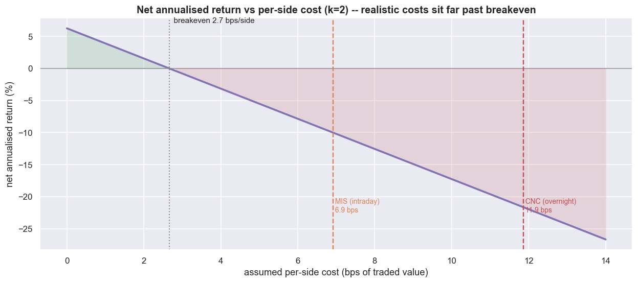
The breakeven cost - the per-side cost at which the strategy exactly stops making money - is 2.66 bps. Realistic intraday cost is 6.9 bps, and overnight is 11.9 bps. So the cheapest you can plausibly trade is more than two and a half times the breakeven. That gap, not any modelling flaw, is the precise reason this is a research model and not a strategy you switch on.

Where this breaks

This signal is real, and it does not pay - both facts are true at once. The verdict for this window and universe: a clean, genuinely market-neutral residual-reversion edge, with a gross Sharpe a little above 1.3 once the sector is removed, that is decisively unprofitable after realistic NSE costs in the form shown here.

• Turnover and costs dominate, full stop. The edge is a few bps per day. Realistic per-side cost is several bps, applied to about 1.0x turnover every day. So the net flips from a gross Sharpe of 1.34 to a net of -1.99. The breakeven of 2.66 bps is a fraction of the 6.9-11.9 bps you can actually trade at. No amount of factor-model polish fixes an edge smaller than its own cost.

• Capacity is tiny, and market impact is assumed away. The cost model uses a flat 2 bps for market impact. But a residual-reversion book demands liquidity exactly when it is scarcest - it buys what just fell and shorts what just ran. Real impact grows with size, so the modest gross edge shrinks as you scale up, while costs do not. Real capacity needs hundreds of names and hard per-name limits, not 50 large caps.

• The short side may not be tradeable. Half the book is short. In India, shorting means one of three things: an intraday cash short (no overnight hold, so you give up the overnight residual), borrowed stock (limited supply, and a fee that eats the thin edge), or single-stock futures (only F&O names, and subject to position-limit bans and roll costs). If you cannot short a name cleanly, the book stops being market-neutral. Treat the short leg as a research abstraction unless you have a real way to put it on.

• Factor crowding and decay. Cross-sectional reversal is one of the best-known, most-traded signals in the world. The edge is thin because so many people chase it. In a forced sell-off it can flip violently into momentum, as every desk unwinds the same residual losers at once - the August 2007 quant quake is the textbook case. A backtested gross Sharpe is a best case that crowding wears down over time.

• Beta-estimation error. "Market-neutral" is only as good as the rolling beta behind it. A 120-day beta is stale after a regime change, noisy for stocks with little history, and wrong around corporate actions. So the residual still carries some leftover market and sector exposure, and the supposedly neutral book quietly takes on directional risk it never accounted for.

• Survivorship bias and a point-in-time universe. This is today's index looking backward. A genuine cross-sectional book trades the membership as it actually changed over time, including names that were later dropped or delisted. Including those would lower the gross signal below what this flattering sample shows.

This is the most scalable idea in the course and, in the same breath, its clearest lesson. The signal is real. The residual genuinely reverts. The book is genuinely neutral. And once you pay realistic NSE costs to harvest it, it is a clean research signal with no tradeable edge left. It only becomes interesting if you can do two things at once: drive per-side cost below about 2.66 bps, and implement the short side for real. Until both are true, the honest description is exactly that - research, not a strategy. The next chapter turns to the risk and sizing machinery that decides whether any of these signals, gross edge and all, can survive as a real book. Educational content only, not investment advice.