What Statistical Arbitrage Really Is

"Arbitrage" usually means a free lunch. You buy the same cash flow cheap in one place and sell it dear in another, at the same moment, and carry no risk in between. Statistical arbitrage keeps the idea but quietly drops the guarantee. Here nothing forces the two prices back together - no shared coupon, no settlement, no rule of law. All you have is a statistical relationship between two assets. In the past it has snapped back often enough, and fast enough, that betting on it again pays off: after costs, most of the time, on average. Every one of those qualifiers is a place the trade can die. This chapter teaches you to see them - and to tell a real relationship from one your eyes invented.

We build up from the floor. First a clean made-up example you can stare at until the mechanics are obvious. Then the same picture on a real NSE pair that the data itself picks out - where, fair warning, it does not behave. After that: how the idea scales to more stocks, what "market neutral" really buys you, and a clear-eyed look at why most of the old edge is gone. Every number below is computed from the data in front of us. It is true in this data window and promised nowhere beyond it.

Trade the relationship, not the price

A single stock price behaves almost like a random walk: tomorrow's price is today's price plus some random noise, with no "home" value pulling it back. So trying to predict the price level is really just trying to predict noise, and that almost never works. Statistical arbitrage gives up on predicting the level. Instead it looks for a combination of two (or more) prices whose difference is stationary - it drifts away from an average and then gets pulled back, over and over. Here is why that can happen. When two stocks are driven by the same forces, each price wanders randomly, but the shared trend cancels out when you subtract one from the other. What's left is a small, mean-reverting wobble. That wobble - not the price - is the thing you trade.

Before touching a real ticker, let us build the perfect case in numpy so the mechanics are clear. We make a shared random-walk trend - it stands in for "whatever moves the whole sector." We add a mean-reverting wobble, an AR(1) process, a simple model of a series where each step leans back toward the average. Price X is the trend plus tiny noise. Price Y is the trend plus the wobble. By construction the two are cointegrated: each one wanders like a random walk on its own, but a particular combination of them, here spread = Y - X, is stationary. It is as if they are tied together by an invisible elastic band. To put a number on it we use the ADF test (Augmented Dickey-Fuller), which asks one simple question: is this series a random walk, or does it mean-revert? It is the workhorse stationarity test used throughout this course.

Copy

from statsmodels.tsa.stattools import adfuller

def half_life(series):
    """Days to revert half a deviation, from an AR(1) fit: delta_t = a + b*level_{t-1}."""
    s = pd.Series(series).dropna().values
    lag, delta = s[:-1], np.diff(s)
    b = np.polyfit(lag, delta, 1)[0]
    return -np.log(2) / np.log(1 + b) if b < 0 else np.nan

rng = np.random.default_rng(7)
n = 750                                            # ~3 trading years
common = 100 + np.cumsum(rng.normal(0, 1.0, n))    # shared random-walk trend
phi, sig = 0.93, 1.2                               # AR(1): slow mean reversion
s = np.zeros(n)
for t in range(1, n):
    s[t] = phi * s[t-1] + rng.normal(0, sig)       # mean-reverting wobble
X = common + rng.normal(0, 0.4, n)                 # price A: trend + tiny noise
Y = common + s                                     # price B: trend + wobble
spread = Y - X
idx = pd.bdate_range('2023-01-02', periods=n)

p_X      = adfuller(X)[1]
p_spread = adfuller(spread)[1]
print(f'ADF p-value on price X     : {p_X:6.3f}  (high -> cannot reject random walk -> NON-stationary)')
print(f'ADF p-value on the spread  : {p_spread:6.3f}  (low  -> reject random walk -> STATIONARY)')
print(f'spread half-life           : {half_life(spread):6.1f} days')

fig, (ax1, ax2) = plt.subplots(2, 1, figsize=(11, 7), sharex=True)
ax1.plot(idx, X, color=C['blue'],  lw=1.6, label='X = trend + noise')
ax1.plot(idx, Y, color=C['amber'], lw=1.6, label='Y = trend + wobble')
ax1.set_title('Two synthetic prices: both wander like random walks'); ax1.legend(loc='upper left')
ax2.plot(idx, spread, color=C['green'], lw=1.4)
ax2.axhline(spread.mean(), color='w', lw=1, ls='--')
ax2.axhline(spread.mean()+2*spread.std(), color=C['red'], lw=0.9, ls=':')
ax2.axhline(spread.mean()-2*spread.std(), color=C['red'], lw=0.9, ls=':')
ax2.set_title('Their spread (Y - X): flat, mean-reverting, stationary  -- this is what we trade')
plt.tight_layout(); plt.show()

Live output

ADF p-value on price X     :  0.465  (high -> cannot reject random walk -> NON-stationary)
ADF p-value on the spread  :  0.000  (low  -> reject random walk -> STATIONARY)
spread half-life           :    8.3 days

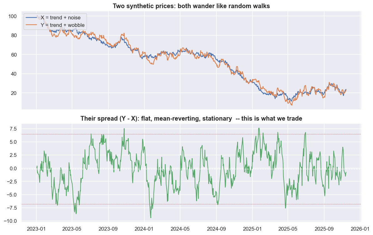
Read the printout, not the picture. The p-value answers one careful question: if the series really were just a random walk, how often would a test come out at least this extreme? Small (below 0.05) is evidence of mean reversion; large means you cannot rule out a random walk. One thing it is not: it is not the probability that the random-walk story is true - only how surprising this data would be if it were. (Chapter 5 has a short statistics primer if any of this is new.) For price X the ADF p-value is 0.465 - high, so we cannot rule out a random walk, and the level really is unforecastable. For the spread the p-value is 0.000 - it clearly rejects the random walk and calls the spread stationary. The spread's half-life is 8.3 days. The half-life is how long a deviation takes, on average, to shrink by half, which is also the natural holding period of the trade. The top panel is hopeless to forecast: both lines climb, fall and drift with no anchor. The bottom panel is a different kind of thing. It wanders around a fixed average, and the dotted bands mark where a trader would bet on a snap-back. Everything else in this course is engineering around finding, trusting and trading that bottom panel.

The same picture on real NSE data

Made-up data was built to behave. Real prices were not. Instead of hand-picking a pretty pair, we let the data choose one for us. Among stocks in the same sector - which gives a real economic reason to move together - and with a long shared history, which pair has the most correlated daily returns? High return-correlation is necessary, but nowhere near enough, for a tradable spread. It is just the honest place to start looking.

The data's pick is BAJFINANCE vs BAJAJFINSV - two financial (NBFC) names, with a return-correlation of 0.824 over a 2473-day window from mid-2016 to mid-2026. Same group, same sector, closely linked businesses. If any pair has a clean spread, surely this one does.

Copy

A, B, sec = cand.loc[0, 'A'], cand.loc[0, 'B'], cand.loc[0, 'sector']
pair = px[[A, B]].dropna()
reb  = pair / pair.iloc[0] * 100

# hedge ratio from OLS on log prices: log A = alpha + beta * log B + spread
lp = np.log(pair)
res   = sm.OLS(lp[A], sm.add_constant(lp[B])).fit()
alpha, beta = res.params['const'], res.params[B]
spread = lp[A] - (alpha + beta * lp[B])
adf_p  = adfuller(spread.dropna())[1]
hl     = half_life(spread)

print(f'Pair chosen by the data : {A}  vs  {B}   (sector: {sec})')
print(f'window                  : {pair.index.min().date()} -> {pair.index.max().date()}  ({len(pair)} days)')
print(f'daily-return corr       : {cand.loc[0, "ret_corr"]:.3f}')
print(f'OLS hedge ratio beta    : {beta:.3f}   (units of log {B} per unit log {A})')
print(f'ADF p-value on spread   : {adf_p:.3f}   ({"stationary at 5%" if adf_p < 0.05 else "CANNOT reject random walk -- not clean"})')
print(f'spread half-life        : {hl:.0f} days')

fig, (ax1, ax2) = plt.subplots(2, 1, figsize=(11, 7), sharex=True)
ax1.plot(reb.index, reb[A], color=C['blue'],  lw=1.4, label=A)
ax1.plot(reb.index, reb[B], color=C['amber'], lw=1.4, label=B)
ax1.set_title(f'{A} vs {B}: rebased to 100 -- they travel together, but not in lockstep'); ax1.legend(loc='upper left')
ax2.plot(spread.index, spread, color=C['green'], lw=1.1)
ax2.axhline(spread.mean(), color='w', lw=1, ls='--')
ax2.axhline(spread.mean()+2*spread.std(), color=C['red'], lw=0.9, ls=':')
ax2.axhline(spread.mean()-2*spread.std(), color=C['red'], lw=0.9, ls=':')
ax2.set_title('Log-price spread (OLS residual): real mean reversion, but messier and prone to regime shifts')
plt.tight_layout(); plt.show()

Live output

Pair chosen by the data : BAJFINANCE  vs  BAJAJFINSV   (sector: NBFC_Fin)
window                  : 2016-06-28 -> 2026-06-25  (2473 days)
daily-return corr       : 0.824
OLS hedge ratio beta    : 1.153   (units of log BAJAJFINSV per unit log BAJFINANCE)
ADF p-value on spread   : 0.199   (CANNOT reject random walk -- not clean)
spread half-life        : 104 days

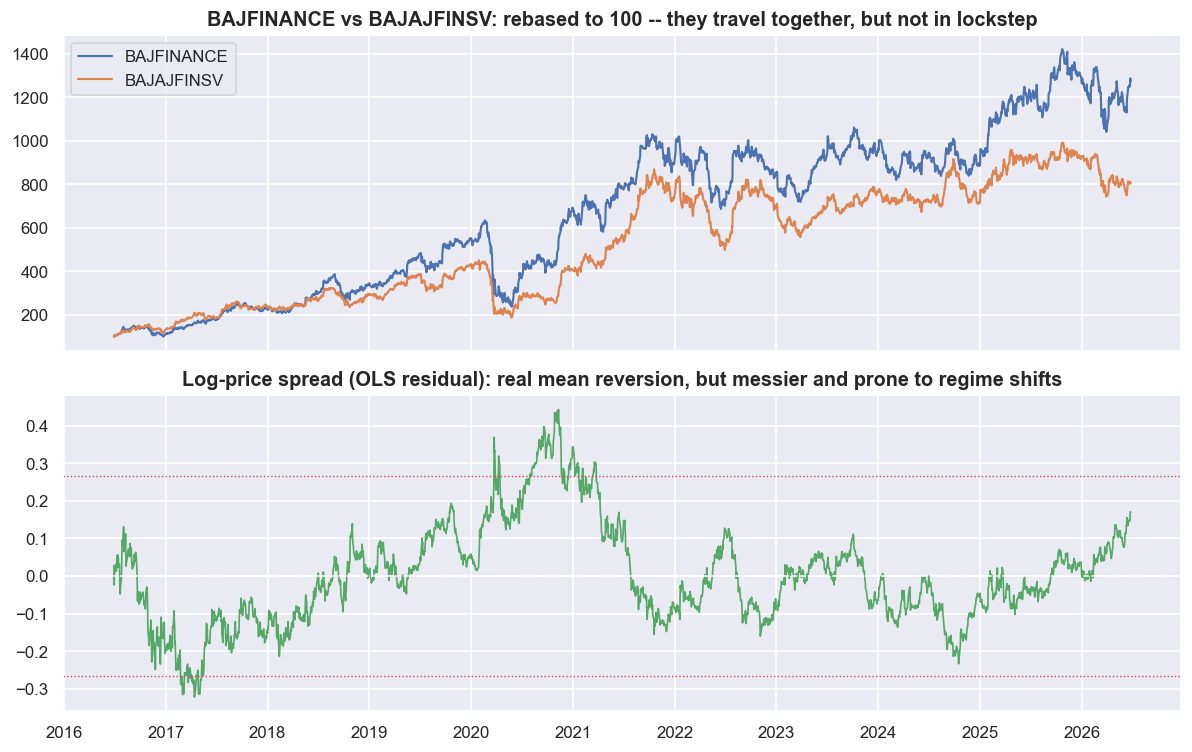
It does not. The two names clearly move together - that is the rebased top panel - but the spread in the bottom panel looks nothing like the made-up one. It swings out far, and its average visibly drifts across the window. The verdict is harsh: the ADF p-value on the spread is 0.199. That is far above 0.05, so we cannot rule out a random walk. The most return-correlated same-sector pair in this whole universe does not give a cleanly stationary spread in this window. And the half-life is 104 days, not the made-up case's tidy eight. Trading this spread means holding a position for months, and that is plenty of time for the relationship to quietly break.

The family tree: one engine, more and more stocks

Pairs trading is the famous version, but it is just one rung on a ladder. As you move up, you add more stocks and remove more directional risk. The underlying bet never changes: a stationary combination drifts away, then reverts.

Single-name reversion trades one series against its own moving average or fair value. It is fragile, because a lone price has no economic reason to come back. Pairs add a second stock and a single hedge ratio (beta) - how many units of stock B you trade against one unit of stock A so their shared market moves cancel. An economic story (same sector, shared input costs) supplies the anchor here. Baskets trade one stock against a weighted basket of its peers - a whole set of weights instead of one ratio - and are sturdier, because a shock to any single peer washes out. Cross-sectional, factor-neutral stat arb ranks the whole universe by a reversion signal, buys the cheap tail, shorts the rich tail, and hedges out sector and market effects. That last form is what the big quant funds actually run. Pairs is the teaching case because you can see every moving part.

Market neutrality: which risk you choose to remove

A long/short book is sold as "market-neutral." But neutrality is a choice about which risk you remove, not something you get for free just by hedging. There are two common targets, and they are not the same.

Dollar-neutral means equal rupees long and short, so your net cash exposure is zero. But if the long leg reacts to the market more strongly than the short leg, the book still rises and falls with the index. You carry a leftover market exposure you never intended. Beta-neutral instead sizes the short leg by the ratio of betas, so the two legs' market moves cancel and only the spread's own behaviour is left - the part you actually wanted. The two are not the same. Let us put numbers on it for our real pair.

Copy

nrets = np.log(nifty).reindex(px.index).diff()

def beta_to_mkt(sym):
    d = pd.concat([rets[sym], nrets], axis=1).dropna(); d.columns = ['s', 'm']
    return sm.OLS(d['s'], sm.add_constant(d['m'])).fit().params['m']

bA, bB = beta_to_mkt(A), beta_to_mkt(B)
h = bA / bB                       # beta-neutral short size on leg B per 1 unit long A
net_dollar = bA - 1.0 * bB        # dollar-neutral (+1 A, -1 B): residual beta
net_beta   = bA - h   * bB        # beta-neutral (+1 A, -h B): ~0 by construction

print(f'market beta of {A:>10}: {bA:.2f}')
print(f'market beta of {B:>10}: {bB:.2f}')
print(f'beta-neutral short size on {B}: {h:.2f}x the long notional')
print(f'net beta  --  dollar-neutral (+1/-1): {net_dollar:+.2f}')
print(f'net beta  --  beta-neutral  (+1/-{h:.2f}): {net_beta:+.2f}')

fig, ax = plt.subplots(figsize=(7.5, 4))
labels = ['Dollar-neutral\n(+1 / -1)', f'Beta-neutral\n(+1 / -{h:.2f})']
sns.barplot(x=labels, y=[net_dollar, net_beta], palette=[C['amber'], C['purple']], ax=ax)
ax.axhline(0, color='w', lw=1)
ax.set_ylabel('residual net market beta'); ax.set_title('Same pair, two neutralities: dollar-neutral still carries index risk')
for i, v in enumerate([net_dollar, net_beta]):
    ax.text(i, v, f'{v:+.2f}', ha='center', va='bottom' if v >= 0 else 'top', color='w', fontweight='bold')
plt.tight_layout(); plt.show()

Live output

market beta of BAJFINANCE: 1.41
market beta of BAJAJFINSV: 1.33
beta-neutral short size on BAJAJFINSV: 1.06x the long notional
net beta  --  dollar-neutral (+1/-1): +0.09
net beta  --  beta-neutral  (+1/-1.06): +0.00

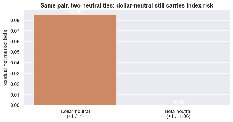
In this window, BAJFINANCE has a market beta of 1.41 and BAJAJFINSV 1.33. Sizing the short at 1.06x the long makes the book beta-neutral. Here is the honest detail. Because these two betas are close, the simple dollar-neutral book (+1 / -1) carries a leftover net beta of only +0.09, while the beta-neutral book sits at +0.00 by design. That small gap is just luck with this particular pair. When the two legs have betas that are far apart, dollar-neutral leaks real index risk, and that leftover can be big enough to drown the spread you were trying to trade. And neither kind of neutrality lasts: betas drift, so a book that is neutral today leaks exposure tomorrow unless you re-hedge - and every re-hedge costs money.

Where the edge came from - and why it decayed

Statistical arbitrage was never magic. In the early days it earned money by providing a service the market needed. When a big buyer pushed one stock above its peers, the arbitrageur sold the expensive one and bought the cheap one. By absorbing that imbalance, they earned the gap as prices came back in line. This is really liquidity provision dressed up as a strategy, and it was the bread and butter of the first quant desks in the late 1980s and 1990s. News also spread slowly back then: it hit the obvious stock first while its peers lagged, and trading that lag paid. On top of that, structural flows - index rebalances, fund redemptions, tax-driven selling - moved spreads for reasons that had nothing to do with fundamentals, and someone got paid to push them back.

Then the edge faded and got crowded. Faster data and faster execution killed the news lag. Thousands of funds now run the same cointegration screens, so deviations get traded away in minutes, not days. Exchange-traded funds and electronic market makers now supply much of the liquidity that pairs traders once sold. More money chasing the same shrinking spread means thinner returns before costs, and a brutal sensitivity to costs. The famous August 2007 "quant quake" - when crowded stat-arb books were forced to unwind into each other over a few days - is the classic proof that this edge is shared, correlated and fragile. The chart below makes the point in miniature: the "relationship" you lean on is not a constant.

Copy

roll = rets[[A, B]].dropna()
rc   = roll[A].rolling(252).corr(roll[B])
fig, ax = plt.subplots(figsize=(11, 4.4))
ax.plot(rc.index, rc, color=C['teal'], lw=1.4)
ax.axhline(rc.mean(), color='w', lw=1, ls='--', label=f'mean {rc.mean():.2f}')
ax.fill_between(rc.index, rc.min(), rc, alpha=0.08, color=C['teal'])
ax.set_title(f'Rolling 1-year return correlation of {A} vs {B}: the "relationship" wanders from '
             f'{rc.min():.2f} to {rc.max():.2f}')
ax.set_ylabel('252-day correlation'); ax.legend(loc='lower left')
plt.tight_layout(); plt.show()
print(f'correlation ranged {rc.min():.2f} -> {rc.max():.2f} over the window; std {rc.std():.2f}.')
print('A pair that is "cointegrated on average" can be uncorrelated for quarters at a time -- exactly when a position is open.')

Live output

correlation ranged 0.71 -> 0.92 over the window; std 0.05.
A pair that is "cointegrated on average" can be uncorrelated for quarters at a time -- exactly when a position is open.

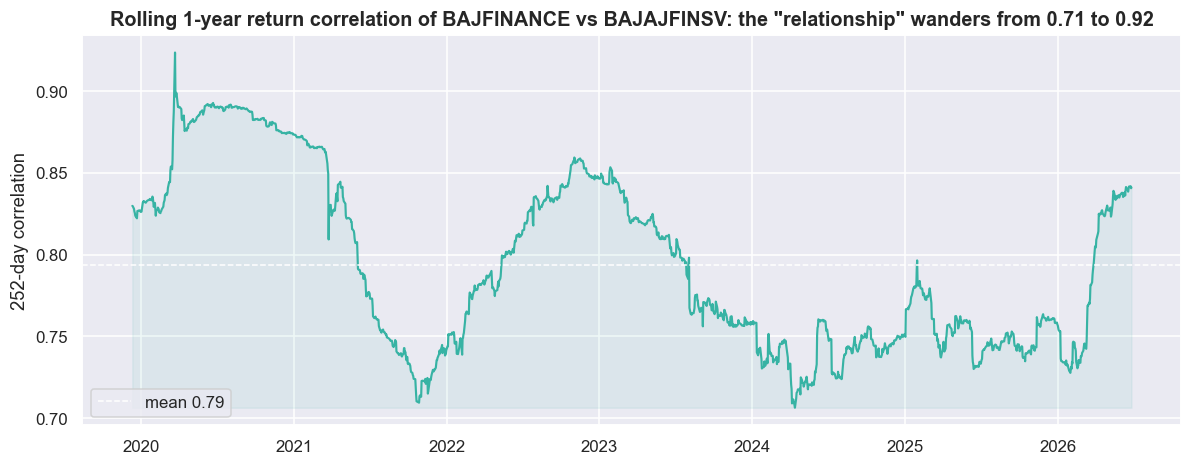
Even our headline pair, which is supposed to move together by nature, has a 1-year rolling return-correlation that ranges from 0.71 to 0.92 across this window, with a standard deviation of 0.05. A pair that looks "cointegrated on average" can be much less linked for quarters at a time - and those quarters are exactly when an open position bleeds. The single average correlation of 0.824 we started with hid all of that movement. Averages flatter you; the timeline tells the truth.

Honest expectations before you go further

Set your expectations correctly now. This is hard, and it is meant to be. The easy spreads are gone. What is left is thin, fast and fought over by better-funded players with faster systems. Costs dominate. Every pair round trip pays statutory charges, spread and market impact - on two legs, on the way in and the way out. A gross edge of a few tens of basis points per trade is routinely negative after costs at retail size. The short leg is rarely free, as noted above. And a statistical relationship existing is not the same as a tradable edge existing. That bright line is the whole reason this module is more than a notebook.

Here is what this series is. Research mechanics first: cointegration, building spreads, designing signals, honest backtesting, and the discipline of testing many ideas without fooling yourself. Execution realism second, layered on top, so you can watch how much of each paper edge survives contact with the real market. The goal is not to sell you a strategy. It is to make you sharp enough to tell a real one from a backtest artefact.

Where this breaks

• A stationary spread in the past guarantees nothing about the future. The ADF and cointegration tests only describe the sample you ran them on. Relationships break on mergers, regulation, capital-structure changes and regime shifts - often right when your position is open. Our chosen pair already failed the test (p = 0.199) in-sample.
• The hedge ratio is estimated, not handed to you. The OLS (ordinary least squares, the standard line-of-best-fit regression) beta of 1.153 is noisy, depends on the look-back window, and drifts. A wrong or stale ratio turns a "market-neutral" spread into a directional bet.
• Return correlation is the wrong test. It is necessary, not sufficient. Two stocks can correlate at 0.824 in returns and still have a non-stationary, untradeable spread. We use it here only to start looking; later chapters replace it with a proper cointegration test.
• Survivorship and point-in-time bias. The universe is today's index members, viewed backwards. Pairs that blew up and were delisted never enter the search, which flatters every statistic.
• Crowding makes the edge correlated across funds. When forced unwinds hit, "market-neutral" books fall together (August 2007). Neutral to the index is not the same as neutral to other arbitrageurs.
• Neutrality leaks. Betas drift, so dollar- or beta-neutral today is not neutral next month without re-hedging - and every re-hedge costs money.

The bottom line: statistical arbitrage is the discipline of trading a stationary relationship you have measured honestly, sized for the risk you chose to keep. You do it knowing the relationship is estimated, decaying, and shared with everyone else running the same screen. The next chapters draw the bright line between a statistical relationship and a tradable edge. They turn the loose word "related" into the precise, testable machinery of cointegration.