Research vs Real Markets

Every chart, test and Sharpe ratio (return divided by risk) in this course is built on the same trade: buy one stock and short another at the closing price. This is a long/short spread - you are long one leg and short the other. The trade works cleanly in a notebook and almost nowhere else.

The long leg is easy. You buy the stock, take delivery, and hold it. The short leg is the hard part. The moment you try to sell a stock you do not own in an Indian account, you hit real rules: forced intraday square-off, hard-to-borrow stock, the futures basis (the gap between a future's price and the cash price), position-limit bans, margin calls, price bands and physical settlement.

None of those frictions show up in a series of closing prices. So none of them show up in a backtest built on closing prices either. Carry this chapter as the lens for every later one. It boils down to one line: a statistical relationship existing is not the same as a tradable edge existing - and almost the whole gap between the two is the short leg.

The backtest makes three quiet assumptions

When a later chapter buys stock A, shorts stock B at the close, and waits for the spread to return to its average, it quietly assumes three things. First, that you can stay short B for as long as the reversion takes - days, sometimes weeks. Second, that both legs fill at the price you measured. Third, that holding the position costs nothing.

All three are false in an Indian account, and each one fails for a clear reason. You cannot hold a plain cash short overnight - the broker closes it for you. You measured the adjusted closing price, but you fill on the next bar at a raw price, paying the bid-ask spread and your own market impact. And the short leg carries a borrow fee, a futures basis, or a roll cost - none of which appear in the price series. The diagram below is the mental model for the whole chapter. A clean research lane runs along the top. The messy real-market lane, where the short leg lands, runs underneath.

Why we learn on the close and can never trade it

The statistics in this course are built on daily closing prices. That choice is right for learning and wrong for trading at the same time. The closing price is the cleanest, most comparable number of the day. There is one auction-settled price per stock, and it is adjusted for splits and dividends so that a corporate action doesn't put a fake jump in the relationship we're trying to measure. It also lines up all fifty names on a single date index - exactly the table a cointegration test wants. (Cointegration means each price wanders on its own, but a particular combination of them stays mean-reverting - as if tied by an invisible elastic band.)

So the close is the right signal to learn on. It is also a price you can never actually trade at. An adjusted close has no bid-ask spread, no depth, and no market impact, and the closing auction may not absorb your size anyway. Your signal fires at the close, but your real fill lands on the next bar at a raw price. Hold both ideas at once: the close is the right thing to model and the wrong thing to trade. That discipline is what this whole module is built on.

The short leg is the whole problem

Carrying a short in India is not one decision. It is a choice among four instruments. Each one swaps the clean stock exposure of the backtest for a different vehicle, and each vehicle brings its own set of frictions.

Read the rows honestly. An intraday cash short lets you sell a stock you do not own, but only for the day. The broker force-closes it near the close. So you cannot carry an overnight reversion pair this way, and you pay the spread-and-impact bill twice every day. SLB - securities lending and borrowing - is the closest match to a true short. You borrow the stock, sell it, buy it back later, and pay an annual borrow fee. But SLB in India is thin and patchy. Many names have little or no stock to borrow, the fee jumps just when everyone wants the same short, and the lender can demand the shares back mid-trade. Stock futures are the realistic default for an overnight position. They are a single, deeply liquid instrument in large names, and you can short them directly. The costs are the basis, a roll cost at every expiry, a fixed lot size that stops you sizing to the rupee, margin, and ban risk. A synthetic short built from options copies the same exposure, but it adds two option legs, the option Greeks, and assignment risk. For a simple linear spread it is rarely worth the trouble.

Here is the uncomfortable part. The hedge ratio - how many units of stock B you trade against one unit of stock A so their shared market moves cancel - was estimated on cash closing prices. You now trade it in a different instrument. That mismatch is tracking error you simply did not have in the backtest.

Which names can you actually short-size?

Being in the F and O (futures and options) segment is necessary but not enough. A stock can be in that segment and still trade too little to take a real position without pushing its own price around. So the first filter is liquidity, not statistics. Rank the universe by average daily traded value - the closing price times volume, in rupees crore. That gives a rough measure of how much size each leg can absorb.

Copy

# Average daily traded value (ADV) over the last ~year, in Rs crore/day.
adv = {}
for s in UNIVERSE:
    try:
        d = load(s)
        adv[s] = (d['close'] * d['volume']).last('365D').mean() / 1e7
    except Exception as e:
        print('skip', s, e)
adv = pd.Series(adv).sort_values(ascending=False)
show = pd.concat([adv.head(12), adv.tail(8)])
sd = show.reset_index(); sd.columns = ['symbol', 'adv']
sd['tier'] = np.where(sd['adv'] >= adv.median(), 'liquid (size-able)', 'thin (short leg breaks)')
fig, ax = plt.subplots(figsize=(11, 8))
sns.barplot(data=sd, x='adv', y='symbol', hue='tier',
            palette={'liquid (size-able)': C['green'], 'thin (short leg breaks)': C['red']},
            dodge=False, ax=ax)
ax.axvline(adv.median(), color=C['amber'], ls='--', lw=1.2)
ax.set_title('Average daily traded value, last ~year (Rs crore) - top 12 and thinnest 8')
ax.set_xlabel('Rs crore traded / day'); ax.set_ylabel(''); ax.legend(loc='lower right')
plt.tight_layout(); plt.show()
print(f'liquidity span in this window: richest {adv.index[0]} ~Rs {adv.iloc[0]:,.0f} cr/day  '
      f'vs thinnest {adv.index[-1]} ~Rs {adv.iloc[-1]:,.0f} cr/day  ->  '
      f'{adv.iloc[0]/adv.iloc[-1]:.0f}x apart')
print(f'median name trades ~Rs {adv.median():,.0f} cr/day; '
      f'{(adv < adv.median()/3).sum()} names trade under a third of the median.')

Live output

liquidity span in this window: richest HDFCBANK ~Rs 2,479 cr/day  vs thinnest TATACONSUM ~Rs 164 cr/day  ->  15x apart
median name trades ~Rs 399 cr/day; 0 names trade under a third of the median.

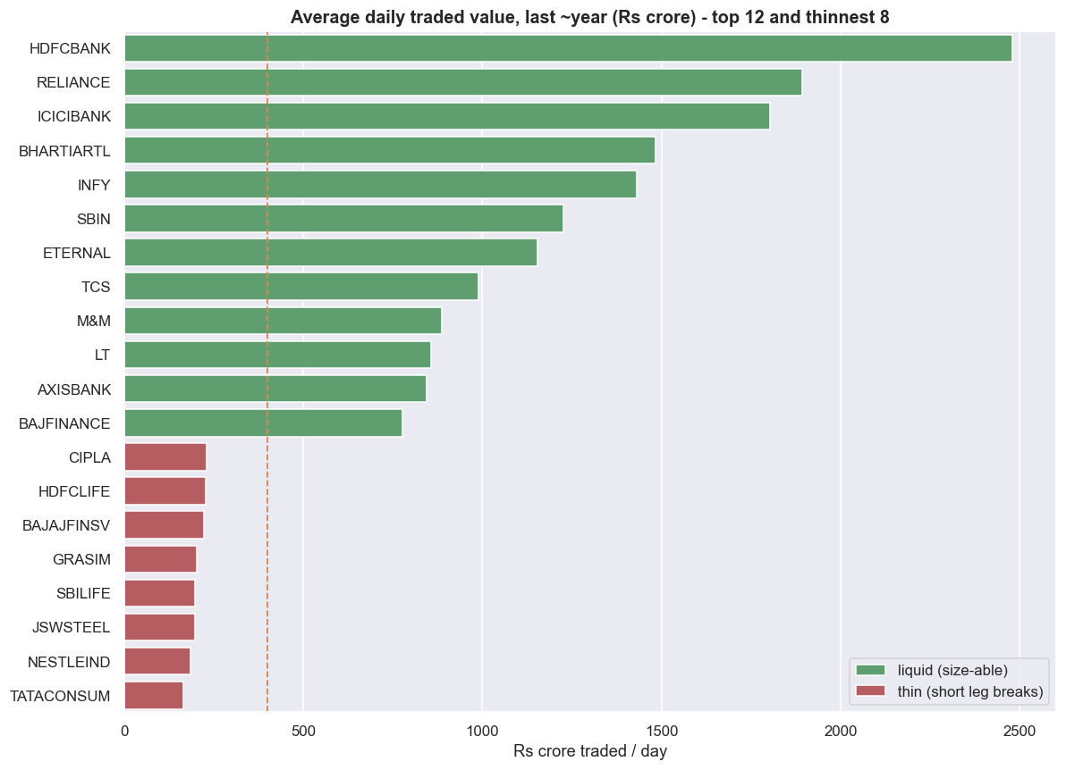
In this data window the busiest name, HDFCBANK, trades about Rs 2,479 crore a day. The thinnest, TATACONSUM, trades about Rs 164 crore - roughly 15x apart inside a single index. The median name trades near Rs 399 crore/day. Notice what this filter does and does not buy you. Because the universe is fifty large caps, no name trades under a third of the median. There is no genuinely untradeable name here. So the filter is discipline, not rescue: it tells you which pairs will cost more in spread, not which ones are impossible. The thin end of the list is still where the short leg quietly breaks - wider spreads, less depth, a less active futures contract, scarcer SLB borrow. And a pair that joins a liquid name to a thin one inherits the thin name's execution problems on both legs.

Eligibility, bans, margin and settlement

Even with a liquid name and a futures contract, four exchange rules decide whether you can hold the trade - and none of them appear in a price series. First, stock futures only exist for names in the F and O segment, and that list is actively managed on liquidity grounds. Names join it and drop off it, and a stock leaving the list kills its futures short outright. Second, the Market-Wide Position Limit (MWPL). When the total open interest across all traders in a stock crosses 95% of its MWPL, the stock enters a ban period. Only trades that reduce positions are allowed. You cannot open or add to a position, and trying draws a penalty. For a market-neutral book this is the worst case. Your pair can be forced into a one-sided exit at exactly the moment the name is most crowded.

The same futures short also brings in margin, price bands and settlement. A short future ties up SPAN plus exposure margin - often a fifth to a third of the notional, per leg. So a pair is two margined legs, both marked to market every day, and a gap day calls for more cash. In practice it is margin, not your signal, that caps your position size. Price bands and circuit limits can freeze a name so you cannot exit one leg - and half a hedge is again naked risk. Settlement also differs by instrument. Cash equity settles T+1. Stock futures are physically settled if you carry them into expiry, so holding a short future to the last day means you owe delivery of the shares. The roll calendar therefore becomes part of the strategy: you must roll or close before every expiry, and you pay the roll cost each month.

The basis you never modelled

When you short a stock through its future, you do not trade the cash price at all. You trade the futures price, which sits away from the spot price by the basis (the gap between the two). Under simple cost-of-carry, the fair futures price is F = S x exp((r - q) x T), where r is the financing rate, q the dividend yield and T the time to expiry. This database has no futures series, so the chart below is a model of the fair basis built off a real spot price, not a market quote. It is just enough to make the size of the basis concrete.

Copy

# Cost-of-carry basis sketch. Real spot, MODELLED basis (no live futures in the DB).
name = 'RELIANCE'
S = float(load(name)['close'].iloc[-1])
r, q = 0.065, 0.006          # illustrative financing rate and dividend yield
days = np.arange(1, 61)
basis = S * np.exp((r - q) * days / 365.0) - S
fig, ax = plt.subplots(figsize=(11, 4.4))
sns.lineplot(x=days, y=basis, color=C['amber'], lw=2, ax=ax)
ax.axhline(0, color=C['grey'], lw=0.8)
ax.set_title(f'{name}: MODELLED fair futures basis vs days to expiry '
             f'(spot Rs {S:,.0f}, r={r:.1%}, q={q:.1%})')
ax.set_xlabel('calendar days to expiry'); ax.set_ylabel('fair basis  F - S  (Rs)')
plt.tight_layout(); plt.show()
b30 = S * np.exp((r - q) * 30/365.0) - S
print(f'~30-day fair basis ~ Rs {b30:,.2f}  ({b30/S*1e4:.1f} bps of spot).')
print('Selling the future to short, this premium converges to zero by expiry - a small')
print('tailwind for the short when r > q, but real quotes also embed demand/borrow and roll cost.')

Live output

~30-day fair basis ~ Rs 6.41  (48.6 bps of spot).
Selling the future to short, this premium converges to zero by expiry - a small
tailwind for the short when r > q, but real quotes also embed demand/borrow and roll cost.

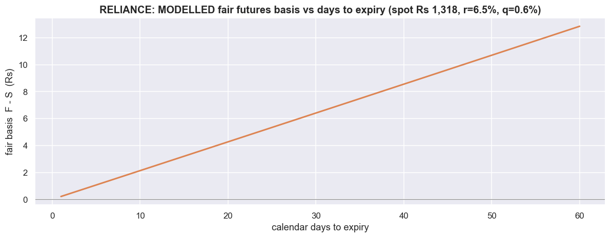
On the real RELIANCE spot price in this window, with an illustrative r = 6.5% and q = 0.6%, the modelled 30-day fair basis is about Rs 6.41, or roughly 48.6 bps of spot. Small - but not zero, and that is the point. The basis changes every day. It shrinks to zero by expiry, which is a mild tailwind for a short when carry is positive. And it appears nowhere in the closing-price series your statistics were built on. So the spread you actually trade on futures is not the spread you tested on cash, and that difference is tracking error. Worse, real futures quotes also bake in demand, borrow scarcity and roll pressure on top of textbook carry. The basis can move against you at exactly the moment a name is hard to borrow - noise your cash-based hedge ratio never saw.

A relationship is not an edge

This is the core idea of the course in one picture. Thousands of pairs move together. Far fewer are cointegrated in-sample - that is, on the data you used to build and tune the model. Fewer still stay cointegrated out-of-sample, on fresh data you never touched. Fewer again survive realistic costs on two legs traded twice. Only what is left at the bottom - cheap to trade, short-able, stable, and net-positive after every layer above - is an actual edge. Each chapter from here adds one more layer to this funnel.

The pre-trade checklist

Before a single rupee of real capital touches a stat-arb idea, the idea has to pass nine gates. A no on any one of them does not mean trade smaller. It means the idea goes back to research, not to the order book.

The gates are not equally famous, but they are equally fatal. Gates 1 to 3 decide whether the trade is even possible: size, short access, and segment-and-ban status. Gates 4 and 5 decide whether it is profitable once the market takes its cut on two legs traded twice - with next-bar fills and the real risk that one leg fills and the other does not. Gates 6 to 9 decide whether you can survive it: margined capital with a gap-day buffer, monitoring that flags a broken leg the moment it happens, a kill switch decided before you need it, and an after-tax view. Futures and cash are taxed differently, and that difference comes straight out of net edge.

Where this breaks

• The short leg is assumed, not guaranteed. Every backtest in this course shorts freely. In a real account the short may have no borrow, be impossible to hold overnight, or sit in an F and O ban exactly when you need it. No short means no market-neutral trade - and that single gate kills more "edges" than any statistical test.
• Instrument mismatch is silent tracking error. Hedge ratios are estimated on cash closing prices but traded in futures, which have their own basis, roll and fixed lot size. The thing you trade is never quite the thing you modelled, and the gap does not show up until real money is on it.
• Costs and carry are off the page. Closing prices contain no spread, no impact, no borrow fee, no basis, no roll and no margin cost. Every one of these subtracts from the curve. This chapter only names them; a later chapter measures the damage.
• Eligibility and limits shift under your feet. F and O membership, MWPL bans, price bands and margin rates all change over time. A relationship that was tradable last year can be off-limits today by rule alone, with no change in the statistics at all.
• This chapter proves nothing on its own. It is judgement and diagrams, not a result. The liquidity numbers are illustrative in this data window, and the basis figure is a model, not a market quote. Carry it as the lens for every later chapter, not as evidence of an edge. The next chapter starts drawing the family tree of the strategy, now that you know which parts of it are research and which parts are real.