The Spread and the Signal

Here is a backtest that returns +98.2% gross, posts a 0.99 Sharpe, wins 72.5% of its trades, and never once hits its stop. (The Sharpe ratio is return divided by risk; higher is better, and below about 1 after costs is weak.) It trades a real NSE pair on real adjusted closes, with honest next-bar fills and no obvious bug. By the end of this chapter you will have built it line by line and watched it work. And you should not believe a single number in it. This is the most seductive chapter in the course, because everything in it is true and almost none of it survives. The whole point is to build a gorgeous in-sample curve on purpose. In-sample means the data we used to fit and tune the model - the data the result is allowed to look good on. We do it cleanly and correctly, every figure computed in this one data window. Then the next chapter takes it apart on fresh data, so you can feel, in your own backtest, exactly how a good-looking result fools the person who built it.

The assembly line: two prices in, one position out

A pairs trade is a short factory line. Prices go in. A hedge ratio - how many units of stock B you trade against one unit of stock A so their shared market moves cancel - collapses the two prices into one spread, the single combined series you actually bet on. A rolling z-score then measures how stretched that spread is right now, in standard deviations from its own recent average. Thresholds turn the z-score into a position. And - the box most backtests quietly skip - the position is filled on the next bar, never the same one. Every section below is one box in this diagram.

The pair is HDFCBANK against KOTAKBANK, two large private banks, chosen because earlier chapters tested it cointegrated and measured its half-life - the time a deviation takes to shrink by half, which sets the natural holding period. A hedge ratio fitted on data that includes the future is a magic trick, not a strategy. So we split time. We estimate everything - the hedge ratio, the spread, its statistics - on a training window of 2019-01-01 to 2023-12-29 (1,239 trading days), and grade it only inside that window for now. The genuine out-of-sample test comes in the next chapter.

First, re-check that the pair is cointegrated on the training window itself, because if it were not, there would be nothing to trade. Engle-Granger returns t = -3.521, p = 0.0306 - cointegrated at the 5% level, in this window. The Step-1 regression A = alpha + beta*B gives a hedge ratio beta = 1.0545 (R-squared 0.83), and the leftover is the spread, s = A - alpha - beta*B, in log units. In plain terms: roughly one unit of HDFCBANK exposure is hedged by about 1.05 units of KOTAKBANK exposure - in this fit.

The spread is not the price ratio

A great deal of "pairs trading" online watches the price ratio, P_A / P_B, and trades when it stretches. That quietly assumes the correct hedge is one rupee of A against one rupee of B - a beta of exactly 1 in log space. Cointegration disagrees. It estimates beta, and the ratio is only the special case where beta happens to equal 1. The way to tell which one is real is stationarity: does the series wander around a fixed average and keep getting pulled back, instead of drifting off forever? So we ADF-test both the ratio and the estimated spread on the training window.

Copy

ratio = (A - B).rename('log price ratio')        # log(P_A / P_B): the implicit beta=1 'spread'
adf_ratio  = adfuller(ratio.dropna(),  autolag='AIC')
adf_spread = adfuller(spread.dropna(), autolag='AIC')
print(f'ADF  log price ratio   (beta=1 implied) : stat = {adf_ratio[0]:+.3f}   p = {adf_ratio[1]:.4f}')
print(f'ADF  cointegrating spread (beta={beta:.3f}) : stat = {adf_spread[0]:+.3f}   p = {adf_spread[1]:.4f}')
print(f"-> {'the estimated spread reverts at least as cleanly' if adf_spread[1] <= adf_ratio[1] else 'similar here (beta is near 1)'} "
      f"(lower p = stronger reversion)")

fig, ax = plt.subplots(2, 1, figsize=(12, 6), sharex=True)
z_r = (ratio - ratio.mean()) / ratio.std()
z_s = (spread - spread.mean()) / spread.std()
sns.lineplot(x=z_r.index, y=z_r.values, color=C['grey'], lw=1.0, ax=ax[0]); ax[0].axhline(0, color=C['amber'], ls='--', lw=1)
ax[0].set_title(f'Log price ratio  log({A_name}/{B_name})  (assumes beta=1)   --   ADF p = {adf_ratio[1]:.3f}')
ax[0].set_ylabel('standardised')
sns.lineplot(x=z_s.index, y=z_s.values, color=C['purple'], lw=1.0, ax=ax[1]); ax[1].axhline(0, color=C['amber'], ls='--', lw=1)
ax[1].set_title(f'Cointegrating spread  A - {beta:.3f}*B  (estimated beta)   --   ADF p = {adf_spread[1]:.3f}')
ax[1].set_ylabel('standardised')
plt.tight_layout(); plt.show()

Live output

ADF  log price ratio   (beta=1 implied) : stat = -3.324   p = 0.0138
ADF  cointegrating spread (beta=1.055) : stat = -3.519   p = 0.0075
-> the estimated spread reverts at least as cleanly (lower p = stronger reversion)

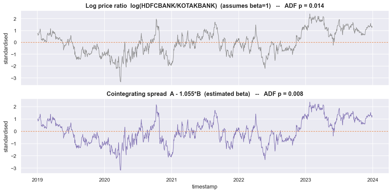
The log price ratio (the implied beta=1 spread) tests at ADF p = 0.0138. The estimated cointegrating spread tests at ADF p = 0.0075 - a lower p, so stronger reversion. Here beta is so close to 1 that the two lines nearly coincide, which is exactly why this is a safe pair to learn on. But do not generalise from how close they look. For a pair whose estimated beta is far from 1, the ratio can wander off and never come back (non-stationary), while the beta-weighted spread reverts cleanly. Letting the ratio pick your hedge is letting a coin flip pick it.

The z-score, and why the window is 29 days

The spread's units - log price - mean nothing to a trader. The z-score rescales it to "how many standard deviations the spread is from its recent average right now." That is directly comparable to a threshold like 2 or 3. Two choices decide everything about how the z-score behaves.

The first is static versus rolling. A static mean and standard deviation, measured over the whole sample, use information from the future, so they leak look-ahead into every early bar. We use a rolling, trailing-only mean and standard deviation instead - computed from past bars only. It adapts to slow drift in the spread, at the cost of being noisier. That is an honest trade-off we are willing to make.

The second is how wide a window. Too short and the z-score is jumpy. Too long and it cannot react. The natural timescale is the spread's half-life - the time it takes to forget half of any deviation. Earlier work measured that at 29.3 days, so we set the rolling window to 29 days. We estimate the spread's recent centre and spread over roughly one half-life. The window is not a free knob we tuned. It is read straight off the spread's own behaviour.

We also build a robust z-score from the rolling median and MAD (median absolute deviation, scaled by 1.4826 to match a normal standard deviation). A single jump wrecks a mean and a standard deviation. The median and MAD shrug it off - and spreads do gap.

Copy

def half_life(s):
    s = pd.Series(s).dropna(); ds = s.diff().dropna(); sl = s.shift(1).dropna()
    sl, ds = sl.align(ds, join='inner')
    kappa = -sm.OLS(ds, sm.add_constant(sl)).fit().params.iloc[1]
    return np.log(2) / kappa if kappa > 0 else np.nan

HL = half_life(spread)
Z_WIN = int(round(HL))                                  # rolling window ~= one half-life
print(f'half-life (notebook 04 method) = {HL:.1f} days  ->  rolling z-score window Z_WIN = {Z_WIN} days')

roll_mean = spread.rolling(Z_WIN).mean()
roll_std  = spread.rolling(Z_WIN).std()
z = ((spread - roll_mean) / roll_std).rename('z')

roll_med = spread.rolling(Z_WIN).median()
roll_mad = spread.rolling(Z_WIN).apply(lambda a: np.median(np.abs(a - np.median(a))), raw=True)
z_robust = ((spread - roll_med) / (1.4826 * roll_mad)).rename('z_robust')

print(f'z (mean/std): mean {z.mean():+.2f}  sd {z.std():.2f}   |   '
      f'z_robust (median/MAD): mean {z_robust.mean():+.2f}  sd {z_robust.std():.2f}')
print(f'correlation between the two z-scores: {z.corr(z_robust):.3f}  '
      f'(close, but the robust one is calmer through gaps)')

fig, ax = plt.subplots(figsize=(12, 4.6))
sns.lineplot(x=z.index, y=z.values, color=C['blue'], lw=1.0, ax=ax, label='z (rolling mean/std)')
sns.lineplot(x=z_robust.index, y=z_robust.values, color=C['amber'], lw=1.0, ax=ax, label='z robust (median/MAD)')
for lvl in [2, -2, 3.5, -3.5]: ax.axhline(lvl, color=C['grey'], ls=':', lw=0.8)
ax.axhline(0, color=C['grey'], ls='--', lw=0.8)
ax.set_title(f'Two z-scores of the {A_name}-{B_name} spread (window {Z_WIN}d ~ one half-life)')
ax.set_ylabel('z'); ax.legend(fontsize=9, ncol=2, loc='upper left')
plt.tight_layout(); plt.show()

Live output

half-life (notebook 04 method) = 29.3 days  ->  rolling z-score window Z_WIN = 29 days
z (mean/std): mean +0.06  sd 1.30   |   z_robust (median/MAD): mean +0.11  sd 1.57
correlation between the two z-scores: 0.948  (close, but the robust one is calmer through gaps)

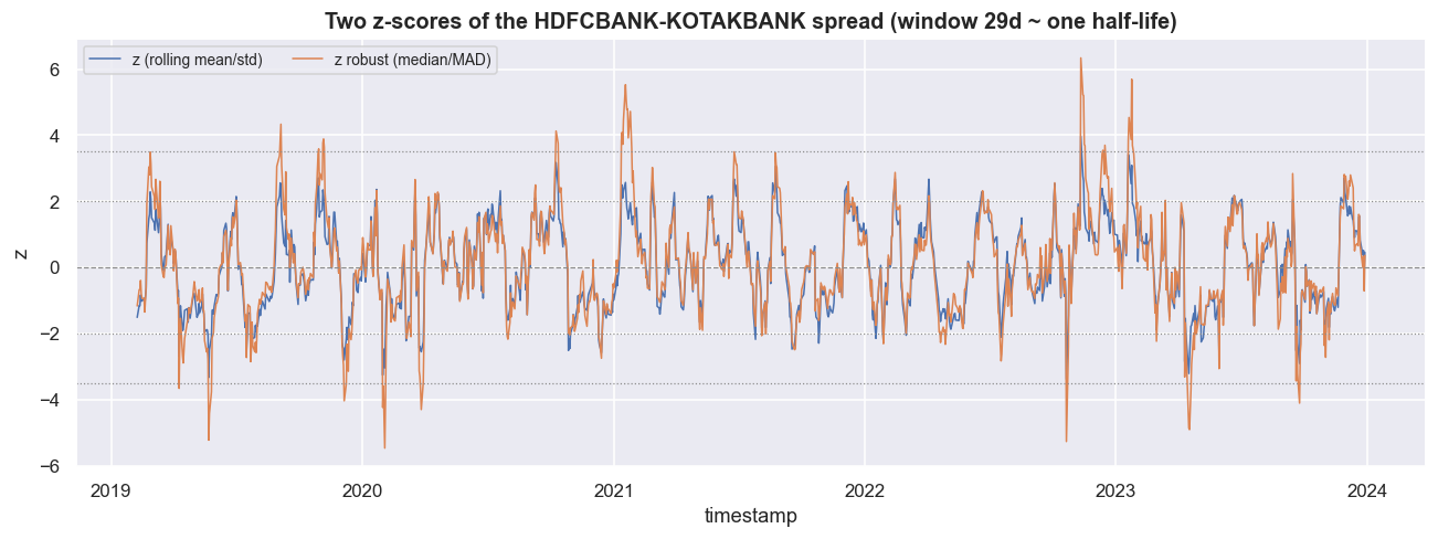
The two z-scores correlate at 0.948 - close, but not identical. The ordinary z has mean +0.06 and standard deviation 1.30. The robust z has mean +0.11 and standard deviation 1.57, running a touch hotter precisely because it refuses to let outliers inflate its spread estimate. Through a clean stretch the two agree. Through a gap, the robust version stays calmer and fires fewer panicked signals.

Four zones: enter, exit, stop

The rules are deliberately simple and symmetric. Enter when 2 < |z| < 3.5: stretched, but not broken. If z is above +2 the spread is rich, so short the spread (short A, long B). If z is below -2 it is cheap, so long the spread (long A, short B). Exit when |z| < 0.5: the spread has come home, so bank it. Hard stop when |z| > 3.5: a move this large usually means the relationship is breaking, not just stretching, so get flat and do not re-enter until z is back inside the band. The z-axis therefore splits into four zones.

Running these rules over the training window decides a position at every close: 262 long-spread bars, 302 short-spread bars, 675 flat bars - and zero hard stops triggered in this window. That last number should make you suspicious, not happy. A strategy that never once hit its stop in five years did not find a magically safe spread. It found a stretch of history kind enough never to push the relationship past breaking. The next window may not be so polite.

Next-bar fills and rupee-neutral sizing

The single most common way a pairs backtest lies is the same-bar fill: computing a signal from today's close, then pretending you also traded at today's close. You cannot. That close has already happened by the time you know the signal. So here is the rule, stated and enforced. The signal is computed at the close of bar t. The position goes on at the close of bar t+1. P&L accrues only from t+1 onward. In code it is a single .shift(1), and it is the whole difference between an honest curve and a fantasy.

Now the sizing. The signal comes from the beta-weighted spread, but how big is each leg? We size the two legs to equal rupee notional - one rupee long, one rupee short - so the book holds equal money on each side and, to first order, cancels market moves. The position is therefore +1 (long spread: +1 rupee A, -1 rupee B), -1 (short spread), or 0 (flat). The per-bar P&L on a +1 book is simply r_A - r_B. With beta at 1.05 here, equal-rupee sizing and exact beta-weighted sizing are almost the same thing. For a pair with beta far from 1 they are not, and the difference leaks back in as directional market exposure. Flagging that gap is the honest move, and we come back to it below.

The curve that is meant to seduce you

Here is the whole strategy in one frame. On top is the spread with its rolling mean and the +/-2 (enter) and +/-3.5 (stop) bands - all moving over time, because the z-score is rolling. Below is the z-score, with the four zones shaded and the actual entries (triangles) and exits (crosses) drawn on the executed bar, one bar after the signal fires.

Copy

entries = pos_exec[(pos_exec != 0) & (pos_exec.shift(1).fillna(0) == 0)].index
exits    = pos_exec[(pos_exec == 0) & (pos_exec.shift(1).fillna(0) != 0)].index

fig, (ax1, ax2) = plt.subplots(2, 1, figsize=(13, 8), sharex=True, gridspec_kw=dict(height_ratios=[1.1, 1]))

# --- top: spread + rolling mean + bands + trade markers
sns.lineplot(x=spread.index, y=spread.values, color=C['purple'], lw=1.0, ax=ax1, label='spread')
ax1.plot(roll_mean.index, roll_mean.values, color=C['grey'], lw=1.1, ls='--', label=f'rolling mean ({Z_WIN}d)')
ax1.plot(roll_mean.index, (roll_mean + 2*roll_std).values,    color=C['amber'], lw=0.9, ls=':')
ax1.plot(roll_mean.index, (roll_mean - 2*roll_std).values,    color=C['amber'], lw=0.9, ls=':', label='+/-2 sd (enter)')
ax1.plot(roll_mean.index, (roll_mean + STOP*roll_std).values, color=C['red'],   lw=0.9, ls=':')
ax1.plot(roll_mean.index, (roll_mean - STOP*roll_std).values, color=C['red'],   lw=0.9, ls=':', label='+/-3.5 sd (stop)')
ax1.scatter(entries, spread.reindex(entries), marker='^', s=60, color=C['green'], zorder=5, label='entry (next-bar fill)')
ax1.scatter(exits,   spread.reindex(exits),   marker='x', s=55, color=C['red'],   zorder=5, label='exit')
ax1.set_title(f'{A_name} - {beta:.3f}*{B_name}: spread with rolling mean and bands')
ax1.set_ylabel('spread (log)'); ax1.legend(fontsize=8, ncol=3, loc='upper left')

# --- bottom: z-score + shaded zones + markers
ax2.set_ylim(-4.5, 4.5)
ax2.axhspan(-EXIT, EXIT, color=C['green'], alpha=0.12)
ax2.axhspan(ENTER, STOP, color=C['amber'], alpha=0.12); ax2.axhspan(-STOP, -ENTER, color=C['amber'], alpha=0.12)
ax2.axhspan(STOP, 4.5, color=C['red'], alpha=0.12);     ax2.axhspan(-4.5, -STOP, color=C['red'], alpha=0.12)
sns.lineplot(x=z.index, y=z.values, color=C['blue'], lw=0.9, ax=ax2)
for lvl in [ENTER, -ENTER, EXIT, -EXIT, STOP, -STOP]: ax2.axhline(lvl, color=C['grey'], ls=':', lw=0.7)
ax2.scatter(entries, z.reindex(entries), marker='^', s=60, color=C['green'], zorder=5)
ax2.scatter(exits,   z.reindex(exits),   marker='x', s=55, color=C['red'],   zorder=5)
ax2.set_title('z-score with shaded zones: green = exit (|z|<0.5), amber = entry (2<|z|<3.5), red = stop (|z|>3.5)')
ax2.set_ylabel('z'); ax2.set_xlabel('')
plt.tight_layout(); plt.show()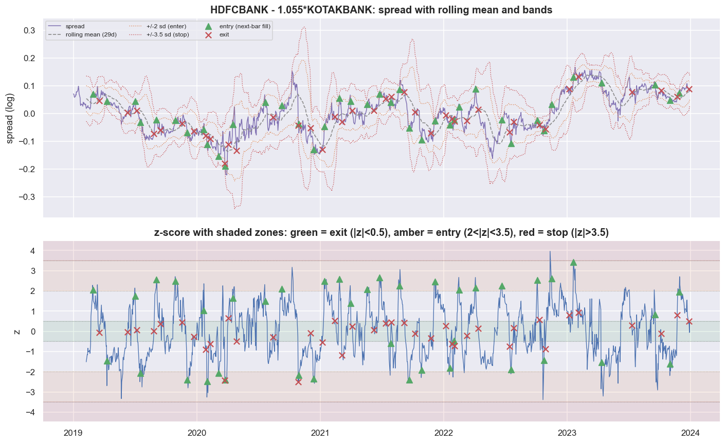

You can read the entire logic off that picture. The spread stretches to a band. An entry triangle appears one bar later. The spread walks back toward its rolling mean. An exit cross lands inside the green zone. Now compound it.

Copy

fig, ax = plt.subplots(figsize=(12, 4.8))
ax.plot(equity.index, equity.values, color=C['green'], lw=1.7, label='strategy equity (gross, in-sample)')
ax.axhline(1.0, color=C['grey'], ls='--', lw=1)
y0, y1 = equity.min()*0.98, equity.max()*1.02
ax.fill_between(pos_exec.index, y0, y1, where=(pos_exec != 0).values, color=C['blue'], alpha=0.06, step='pre',
                label='in market')
ax.set_ylim(y0, y1)
ax.set_title(f'In-sample equity curve  ({A_name}/{B_name}, gross of costs)')
ax.set_ylabel('growth of 1 (per-leg notional)'); ax.legend(fontsize=9, loc='upper left')
plt.tight_layout(); plt.show()

roll_max = equity.cummax(); dd = equity/roll_max - 1
print(f'max drawdown (in-sample, gross): {dd.min():.1%}')

Live output

max drawdown (in-sample, gross): -18.8%

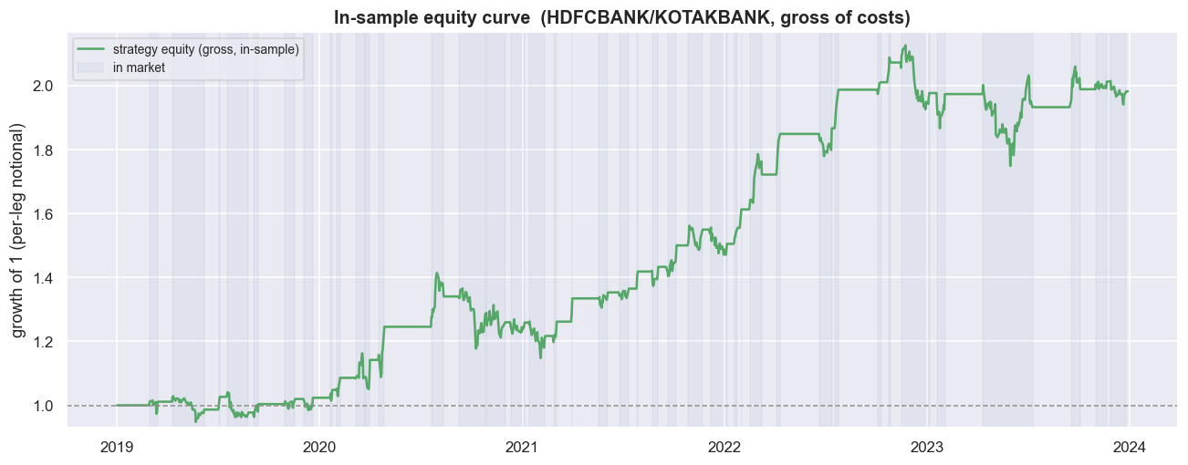
One unit of the rupee-neutral book grows to +98.2% gross over the window, at an annualised Sharpe of 0.99, with a maximum drawdown of -18.8% and 46% time in market. Notice the shape. The curve is flat whenever the book is flat, and it earns in bursts when a stretched spread snaps back. That is exactly what mean reversion should look like - which is part of what makes it so convincing. The trade ledger backs it up: 40 round trips, a 72.5% hit rate, +1.78% average trade, average winner +3.42% against average loser -2.54%, held about 14 days each.

Copy

fig, ax = plt.subplots(1, 2, figsize=(13, 4.4))
sns.histplot(trades.trade_ret*100, bins=18, kde=True, color=C['blue'], ax=ax[0])
ax[0].axvline(0, color=C['red'], ls='--', lw=1.2)
ax[0].axvline(avg*100, color=C['green'], ls='-', lw=1.6, label=f'mean {avg*100:+.2f}%')
ax[0].set_title('Per-trade return (in-sample, gross)'); ax[0].set_xlabel('trade return (%)'); ax[0].legend(fontsize=9)
sns.histplot(trades.days, bins=15, color=C['amber'], ax=ax[1])
ax[1].axvline(HL, color=C['purple'], ls='--', lw=1.6, label=f'half-life {HL:.0f}d')
ax[1].set_title('Holding period'); ax[1].set_xlabel('days held'); ax[1].legend(fontsize=9)
plt.tight_layout(); plt.show()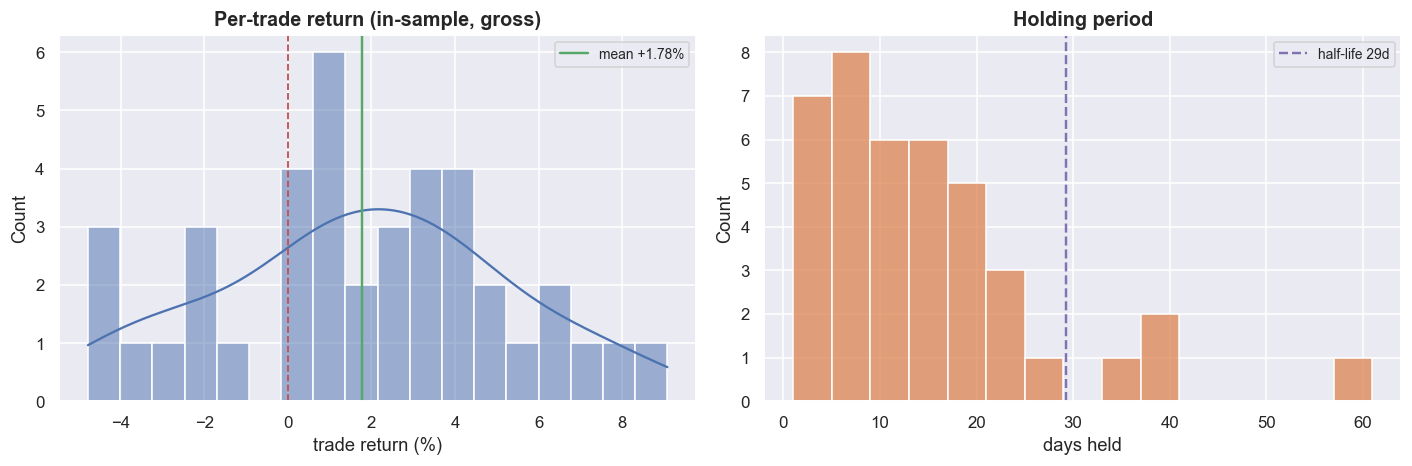

The trade distribution is textbook mean reversion: a tight cluster of small wins, a thin left tail of larger losses, and holding periods scattered around the 29-day half-life - exactly why the z-score window was tied to it. By every conventional metric on the page, this is a strategy you would fund.

It is not. We even peeked at costs. One pair round trip - two legs, in and out - runs roughly 28 bps of leg notional, and 40 of them stack to about an 11% additive drag against the +98% gross. That alone does not kill it. But cost is the smallest of the problems here, and stacking the rest up is the entire job of the next chapter.

Where this breaks

This curve is designed to look good, and it stands on five soft spots the next chapter presses until they crack.

• It is in-sample. The beta, the half-life, the window and the thresholds were all fitted or chosen inside 2019-2023. The only honest grade is out-of-sample, and we have not run it yet. Expect most of the +98% and most of the 0.99 Sharpe to belong to the training data, not the strategy.
• It is gross of costs. Every round trip crosses the bid-ask spread on two legs, twice, and pays the full statutory stack. The back-of-envelope drag is ~11% here. The honest net curve, with slippage and market impact, is heavier and comes later.
• Beta is frozen, but it drifts. We froze a single in-sample hedge ratio. Out-of-sample it will be the wrong number, the spread will mis-hedge, and the bands will be breached for reasons that have nothing to do with reversion. Later chapters let beta change over time.
• Rupee-neutral is not exactly the cointegrating hedge. Equal-rupee sizing matches the beta-weighted hedge only because beta is near 1 in this window. For a different pair, the leftover market exposure leaks in as directional P&L that has nothing to do with the spread.
• The short leg is a research abstraction. The whole book assumes cheap, reliable shorting of a single stock for weeks at a time. In Indian markets that means intraday cover, borrowed stock or a futures proxy - each with costs, margin and availability that are absent from this equity-price backtest.

Zero hard stops, a 72% hit rate and a near-doubling of capital are not evidence the strategy works. They are evidence the window was kind and the grader was the strategy's own teacher. Everything here is true, in this data window, gross, in-sample - and that sentence is the trap the next chapter springs.