The Brutal Reality Check
Take the pretty backtest apart: out-of-sample collapse, realistic NSE costs net of gross, the spread de-cointegrating, and look-ahead, with the losing net curve shown, not hidden.
- ·Out-of-sample collapse
- ·Real NSE costs, gross vs net
- ·Rolling de-cointegration
- ·Look-ahead quantified
- ·Survivorship in pair selection
- ·The honest verdict
Here is the curve that gets a strategy funded. In the last chapter we built a pairs trade on HDFCBANK and KOTAKBANK. First we pick a hedge ratio - how many units of one stock we trade against one unit of the other so their shared market moves cancel - and freeze it. Then we track the spread, the gap left after subtracting one stock from the other. The z-score tells us how far that spread sits from its own average, measured in standard deviations. We enter when the z-score hits plus or minus two, exit at the average, and hard-stop at four. Run that over 2019 to 2023 and it prints a net Sharpe of 1.01 (Sharpe is return divided by risk, where higher is better). Total return is +110.5%, with drawdowns shallow enough to sleep through. Twenty-two clean round trips. It looks like money.
This chapter takes that exact curve apart, the way a risk committee would before risking a single rupee. A backtest is only a hypothesis dressed up as a result. Between the pretty chart and a real profit-and-loss sit four leaks. We will open each one on the same pair, with the real numbers, in this data window.
Four leaks between a chart and a P&L
Keep one picture in mind for the whole chapter. The top line is the curve a naive backtest prints. The bottom line is what you could actually have kept. Every gap between them is one of four leaks - not real edge. The rest of the chapter just measures each gap on real data.
A few honesty rules are baked in before we start, so we are not fooling ourselves on the first page. The hedge ratio b = 1.0545 is estimated on the train window only, then frozen. The test period never touches it. The z-score is trailing: it uses a rolling 60-day window (about two half-lives), so the signal at any moment only sees past data. The half-life is how long a deviation takes to shrink by half, which in practice is the natural holding period of the trade. The fill is next-bar: the signal forms at today's close, and the trade is executed on the next bar. Costs are delivery (CNC) costs, and a round trip is 0.474% of notional. We use delivery costs because a roughly 29-day half-life means positions are held for weeks, not squared off intraday. With those rules fixed, we open the leaks.
Teardown one: the edge does not survive a blind window
The single most important question about any backtest is simple. Does the rule still work on data it was not built on? That fresh, untouched data is called out-of-sample data - the only honest test of a model. We froze the hedge ratio and the thresholds on 2019 to 2023. Then we applied them, completely unchanged, to 2024 to now - data the model has never seen.
g_oos, n_oos = perf(bt['gross'].loc[ooS]), perf(bt['net'].loc[ooS])
ni, no = eqc(bt['net'].loc[isS]), eqc(bt['net'].loc[ooS])

fig, ax = plt.subplots(figsize=(12, 5.2))
ax.plot(ni.index, ni.values, color=C['blue'], lw=2.0,
        label=f'IN-SAMPLE net   Sharpe {n_is["sharpe"]:.2f}   {n_is["total"]*100:+.0f}%')
ax.plot(no.index, no.values, color=C['red'], lw=2.0,
        label=f'OUT-OF-SAMPLE net   Sharpe {n_oos["sharpe"]:.2f}   {n_oos["total"]*100:+.0f}%')
ax.axvline(pd.Timestamp(OO0), color=C['grey'], ls='--', lw=1.2)
ax.text(pd.Timestamp(OO0), ax.get_ylim()[1]*0.98, '  frozen rule applied blind ->',
        color=C['grey'], fontsize=10, va='top')
ax.axhline(1, color=C['grey'], lw=0.8, ls=':')
ax.set_title('Teardown 1 -- fit on TRAIN, freeze, apply UNCHANGED to the held-out TEST')
ax.set_ylabel('growth of Rs 1 (each leg rebased)'); ax.legend(loc='upper left', fontsize=10)
plt.tight_layout(); plt.show()

drop = (1 - n_oos["sharpe"]/n_is["sharpe"]) * 100
print(f'in-sample  net Sharpe {n_is["sharpe"]:.2f}  ->  out-of-sample net Sharpe {n_oos["sharpe"]:.2f}   '
      f'({drop:.0f}% of the edge gone)')
print(f'out-of-sample: {trips(bt, ooS)} round trips, net total {n_oos["total"]*100:+.1f}% over '
f'{(pd.Timestamp(OO1)-pd.Timestamp(OO0)).days/365.25:.1f} years, max drawdown {n_oos["maxdd"]*100:.1f}%')in-sample net Sharpe 1.01 -> out-of-sample net Sharpe 0.34 (66% of the edge gone) out-of-sample: 11 round trips, net total +11.5% over 2.5 years, max drawdown -13.8%
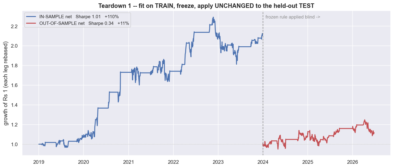
The data the model was built and tuned on is called in-sample data. In-sample, the net Sharpe was 1.01. Out of sample, it falls to 0.34 - about two-thirds of the edge gone. That leaves +11.5% over two and a half years across just 11 round trips, with a -13.8% drawdown. The shape of the curve changes too. The smooth in-sample climb becomes a sideways grind that happens to end up. This is not a strategy that "still works a bit". It is a strategy whose headline number was mostly an artefact of the window it was tuned on.
There is a fairer test. Every quarter, re-estimate the hedge ratio on the trailing two years, then trade the next quarter forward. This is still strictly out-of-sample, but it lets the model keep up as the relationship drifts. This walk-forward approach lands at Sharpe 0.62 overall and +22.3% across 2024 onward (the only genuinely recent slice). It recovers some of the loss. But it still sits far below 1.01, and every refit is one more chance to overfit. Re-estimating is not a free lunch.
The in-sample curve was a hypothesis, not a result. Tested on fresh data, the net Sharpe fell by roughly 66% in this window. So treat any single backtested Sharpe shown without an out-of-sample number beside it as the optimistic end of a range, not the answer.
Teardown two: costs are not a footnote
A pair round trip is not one trade. It is eight fills: two legs, each bought and sold, on entry and again on exit. Every fill pays statutory charges (securities transaction tax, exchange and regulator fees, GST, stamp duty). On top of that, each fill pays half the bid-ask spread it crosses, plus its own market impact. For a multi-week delivery hold, the biggest cost is the 0.1% transaction tax on the sell side. There is no cheap intraday square-off to dodge it.
g_f, n_f = perf(bt['gross'].loc[fullS]), perf(bt['net'].loc[fullS])
gf, nf = eqc(bt['gross'].loc[fullS]), eqc(bt['net'].loc[fullS])
cost_paid = (bt['turn'].loc[fullS] * COST_TURN).sum()      # total fraction lost to costs

fig, ax = plt.subplots(figsize=(12, 5.2))
ax.plot(gf.index, gf.values, color=C['green'], lw=2.0, label=f'GROSS   Sharpe {g_f["sharpe"]:.2f}   +{g_f["total"]*100:.0f}%')
ax.plot(nf.index, nf.values, color=C['blue'],  lw=2.0, label=f'NET of NSE costs   Sharpe {n_f["sharpe"]:.2f}   +{n_f["total"]*100:.0f}%')
ax.fill_between(gf.index, nf.values, gf.values, color=C['red'], alpha=0.12, label='eaten by costs')
ax.axhline(1, color=C['grey'], lw=0.8, ls=':')
ax.set_title('Teardown 2 -- the same strategy, gross vs net of realistic NSE costs (full sample)')
ax.set_ylabel('growth of Rs 1'); ax.legend(loc='upper left', fontsize=10)
plt.tight_layout(); plt.show()

print(f'full sample: {trips(bt, fullS)} round trips x {COST_RT*100:.3f}% = {cost_paid*100:.1f}% of capital paid as costs')
print(f'Sharpe  gross {g_f["sharpe"]:.2f}  ->  net {n_f["sharpe"]:.2f}     '
      f'total return  +{g_f["total"]*100:.0f}%  ->  +{n_f["total"]*100:.0f}%')
print(f'in this window costs are a haircut, not a guillotine -- because +/-2 sd trades rarely. But that')
print(f'depends entirely on the cost you ASSUME. The next chart sweeps it.')full sample: 33 round trips x 0.474% = 15.9% of capital paid as costs Sharpe gross 0.90 -> net 0.77 total return +175% -> +135% in this window costs are a haircut, not a guillotine -- because +/-2 sd trades rarely. But that depends entirely on the cost you ASSUME. The next chart sweeps it.
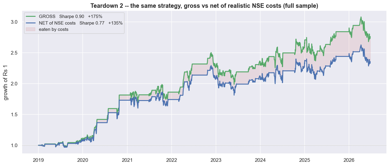
Over the full sample that is 33 round trips times 0.474% = 15.9% of capital paid away as costs. The difference between two numbers matters here: gross is the return before costs, net is after, and stat arb lives or dies on net. Here the gross Sharpe of 0.90 becomes a net 0.77, and the total return of +175% becomes +135%. In this window costs are a haircut, not a guillotine - mostly because a plus-or-minus-two-standard-deviation rule trades rarely. But that verdict rests entirely on the cost you assume. The half-spread and the impact are the two numbers you can least defend in advance. They move with your size, the time of day, and how the order book looks when you actually trade.
So instead of trusting one cost number, sweep across many. As the assumed round-trip cost rises, the out-of-sample net Sharpe reaches zero at about 1.9% per round trip. And the out-of-sample line sits much closer to that zero axis than the in-sample line does the whole way along. The cushion that looks comfortable in-sample is much thinner once you are out of sample. Your break-even is not a distant cliff. It is roughly four times the cost you hope to pay, and a bad fortnight of fills can spend that margin.
The cost verdict depends on an assumption you cannot pin down before you trade. When a strategy flips from profit to loss somewhere between a 0.5% and a 2% round-trip cost, "is it profitable?" is the wrong question. The right one is "how sure am I of the 0.474%, and what happens if I am wrong by a factor of two?"
Teardown three: the relationship was never stable
Teardown one showed the edge fades out of sample. This teardown shows why. The whole strategy rests on cointegration. On its own, each price behaves like a random walk - tomorrow's price is today's plus random noise, with no home value pulling it back. But a particular combination of the two prices is stationary: it wanders around a fixed average and keeps getting pulled back, instead of drifting off forever. It is as if the two stocks are tied together by an invisible elastic band. That tie is what gives us one stable hedge ratio and a spread that always comes home. We can test whether the tie still holds with a rolling Engle-Granger p-value - the chance, if the pair really were not tied together, of seeing a result at least this extreme. A small p-value (below 0.05) is evidence the pair is cointegrated right now. So we ask the question directly: is the pair cointegrated right now?
def rolling_coint_p(la, lb, w=252, step=10):
    out = {}
    for i in range(w, len(la), step):
        try: out[la.index[i]] = coint(la.iloc[i-w:i], lb.iloc[i-w:i])[1]
        except Exception: pass
    return pd.Series(out)

rc = rolling_coint_p(la, lb)
fig, ax = plt.subplots(figsize=(12, 5.0))
ax.plot(rc.index, rc.values, color=C['purple'], lw=1.6)
ax.axhline(0.05, color=C['red'], ls='--', lw=1.4, label='5% significance')
ax.fill_between(rc.index, 0, 0.05, color=C['green'], alpha=0.10, label='cointegrated zone (p<0.05)')
ax.axvspan(pd.Timestamp(TR0), pd.Timestamp(TR1), color=C['blue'], alpha=0.06, label='TRAIN')
ax.axvspan(pd.Timestamp(OO0), pd.Timestamp(OO1), color=C['amber'], alpha=0.06, label='TEST')
ax.set_ylabel('Engle-Granger p-value (252d rolling)'); ax.set_ylim(0, 1)
ax.set_title('Teardown 3 -- the pair is only "cointegrated" some of the time')
ax.legend(fontsize=8, ncol=2, loc='upper left')
plt.tight_layout(); plt.show()

frac = (rc > 0.05).mean() * 100
print(f'rolling cointegration p-value: min {rc.min():.3f}  max {rc.max():.3f}  latest {rc.iloc[-1]:.3f}')
print(f'the pair FAILS the 5% cointegration test in {frac:.0f}% of rolling windows -- it is the exception,')
print(f'not the rule, that this pair reverts. The clean p=0.03 in notebook 04 was one lucky window.')rolling cointegration p-value: min 0.005 max 0.978 latest 0.734 the pair FAILS the 5% cointegration test in 90% of rolling windows -- it is the exception, not the rule, that this pair reverts. The clean p=0.03 in notebook 04 was one lucky window.
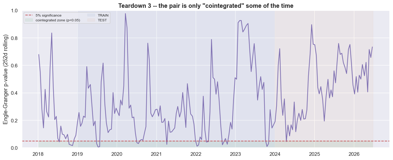
The rolling p-value runs from a low of 0.005 to a high of 0.978, and it sits at 0.734 in the latest window. A value that high means we cannot rule out that the pair is just drifting apart. In fact, the pair fails the 5% cointegration test in about 90% of rolling windows. For this pair, reversion is the exception, not the rule. The clean, tradeable cointegration the build chapter found was one lucky stretch of data, not a permanent property of the two names.
There is a mechanical cause behind this. The hedge ratio is not a constant. The rolling 120-day b swings from -0.312 to 1.744, with a mean of 0.649 and a standard deviation of 0.417. That is a wander of 317% of its own mean, and it even turns negative. When it goes negative, the "hedge" inverts and both legs point the same way. The frozen train value of 1.0545 sits about +63% above the test-period average. So out of sample, the spread we trade is mis-hedged by construction. It carries directional bank-sector risk that has nothing to do with mean reversion. That leaked directional risk is exactly what shows up as the out-of-sample drawdowns.
De-cointegration is not a separate problem from the out-of-sample collapse. It is the engine of it. A fixed hedge ratio trades a snapshot of a relationship that has already ended. When the spread fails the cointegration test in nine windows out of ten, you are not trading an elastic band that occasionally stretches. You are trading a directional bet that occasionally happens to revert.
Teardown four: leaks that flatter quietly
The first three leaks are about the future being unknowable. The fourth is different. It is about the future quietly leaking into the past inside your own code - and about the pairs you never see. The most dangerous version is a normalisation leak. You standardise the spread using the whole sample's mean and standard deviation, instead of a trailing past-only window. It looks like harmless scaling. But that scaling factor secretly contains the test period's own range. So the held-out test is no longer blind.
# A subtler, classic look-ahead: normalise the z-score with WHOLE-SAMPLE mean/std (which "knows"
# the test period's range) instead of a trailing window. This one flatters the held-out test.
z_leak  = (spread - spread.mean()) / spread.std()          # peeks at the future
b_leak  = backtest(beta, z=z_leak)
p_leak  = perf(b_leak['net'].loc[ooS])
p_honest = perf(bt['net'].loc[ooS])
el, eh = eqc(b_leak['net'].loc[ooS]), eqc(bt['net'].loc[ooS])

fig, ax = plt.subplots(figsize=(12, 5.0))
ax.plot(el.index, el.values, color=C['red'],  lw=2.0, label=f'full-sample z (leak)   OOS Sharpe {p_leak["sharpe"]:.2f}   {p_leak["total"]*100:+.0f}%')
ax.plot(eh.index, eh.values, color=C['blue'], lw=2.0, label=f'trailing z (honest)   OOS Sharpe {p_honest["sharpe"]:.2f}   {p_honest["total"]*100:+.0f}%')
ax.axhline(1, color=C['grey'], lw=0.8, ls=':')
ax.set_title('Teardown 4b -- normalising the test set with statistics that include the test set')
ax.set_ylabel('growth of Rs 1 (OOS only)'); ax.legend(loc='upper left', fontsize=10)
plt.tight_layout(); plt.show()

print(f'OOS net Sharpe inflates from {p_honest["sharpe"]:.2f} (trailing, honest) to {p_leak["sharpe"]:.2f} '
      f'(full-sample z) -- a {p_leak["sharpe"]/p_honest["sharpe"]:.1f}x boost from a single subtle leak,')
print('and not a rupee of it is tradeable: you cannot standardise today by a mean you only learn next year.')OOS net Sharpe inflates from 0.34 (trailing, honest) to 1.12 (full-sample z) -- a 3.3x boost from a single subtle leak, and not a rupee of it is tradeable: you cannot standardise today by a mean you only learn next year.
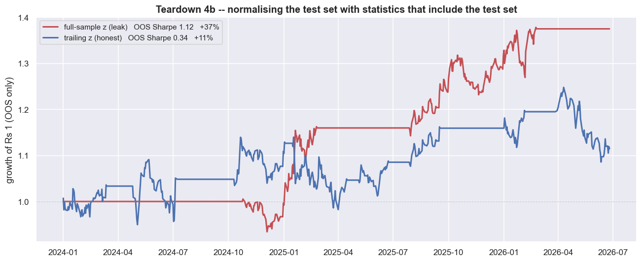
Switching the trailing z-score for a full-sample one lifts the out-of-sample net Sharpe from 0.34 to 1.12 - a 3.3x boost from one subtle leak. Not a rupee of it is tradeable, because you cannot standardise today using statistics you only learn next year. The fill assumption matters just as much. A same-bar fill returns -64% (Sharpe -0.70), against the next-bar +135% (Sharpe 0.77). Notice the direction. For a mean-reversion entry, the same-bar "cheat" is actually worse, because it books the very move that triggered the entry against you. The lesson is not that look-ahead always flatters. It is that a one-day shift in an assumption can move the result by more than the entire edge, in either direction.
Then there is the pair itself. We did not stumble onto HDFCBANK / KOTAKBANK. The build process scanned ten bank pairs and crowned the one that tested most cointegrated in 2019 to 2023. That is selection, and selection has a price.
import itertools
bankpx = closes(SECTORS['Banks'], start='2017-01-01', end='2026-06-26').dropna()

def pair_net_sharpes(Pa, Pb):
    laa, lbb = np.log(Pa), np.log(Pb)
    bb = np.polyfit(lbb.loc[TR0:TR1].values, laa.loc[TR0:TR1].values, 1)[0]
    s  = laa - bb * lbb
    held = positions(zscore(s)).shift(1)
    net  = held * (Pa.pct_change() - bb * Pb.pct_change()) - COST_TURN * held.diff().abs().fillna(0)
    return perf(net.loc[isS])['sharpe'], perf(net.loc[ooS])['sharpe']

rows = []
for a, b in itertools.combinations(SECTORS['Banks'], 2):
    si, so = pair_net_sharpes(bankpx[a], bankpx[b])
    rows.append((f'{a}/{b}', si, so))
sc = pd.DataFrame(rows, columns=['pair', 'IS_net_Sharpe', 'OOS_net_Sharpe']).sort_values('OOS_net_Sharpe')

fig, ax = plt.subplots(figsize=(12, 6.0))
yp = np.arange(len(sc))
ax.barh(yp - 0.2, sc['IS_net_Sharpe'],  height=0.4, color=C['blue'], label='in-sample net Sharpe')
ax.barh(yp + 0.2, sc['OOS_net_Sharpe'], height=0.4, color=C['red'],  label='out-of-sample net Sharpe')
ax.set_yticks(yp); ax.set_yticklabels(sc['pair'])
ax.axvline(0, color=C['grey'], lw=1.0)
for i, pr in enumerate(sc['pair']):
    if pr == f'{A_name}/{B_name}':
        ax.axhspan(i-0.45, i+0.45, color=C['amber'], alpha=0.12)
ax.set_xlabel('net Sharpe'); ax.set_title('Teardown 4c -- survivorship: we picked the IN-SAMPLE winner of 10 bank pairs')
ax.legend(fontsize=9, loc='lower right')
plt.tight_layout(); plt.show()

our = sc[sc['pair'] == f'{A_name}/{B_name}'].iloc[0]
print(f'{A_name}/{B_name}:  IS net Sharpe {our["IS_net_Sharpe"]:.2f} (rank '
      f'{int((sc["IS_net_Sharpe"]>our["IS_net_Sharpe"]).sum())+1} of {len(sc)} in-sample)  '
      f'->  OOS net Sharpe {our["OOS_net_Sharpe"]:.2f}')
print(f'{(sc["OOS_net_Sharpe"]<0).sum()} of {len(sc)} bank pairs actually LOSE money net out-of-sample.')
print('We did not find a good pair; we ran a beauty contest in-sample and crowned a winner. Out of sample,')
print('the crown is worth little -- and the pairs that broke (and the names that delisted entirely) are invisible here.')HDFCBANK/KOTAKBANK: IS net Sharpe 1.01 (rank 1 of 10 in-sample) -> OOS net Sharpe 0.34 5 of 10 bank pairs actually LOSE money net out-of-sample. We did not find a good pair; we ran a beauty contest in-sample and crowned a winner. Out of sample, the crown is worth little -- and the pairs that broke (and the names that delisted entirely) are invisible here.
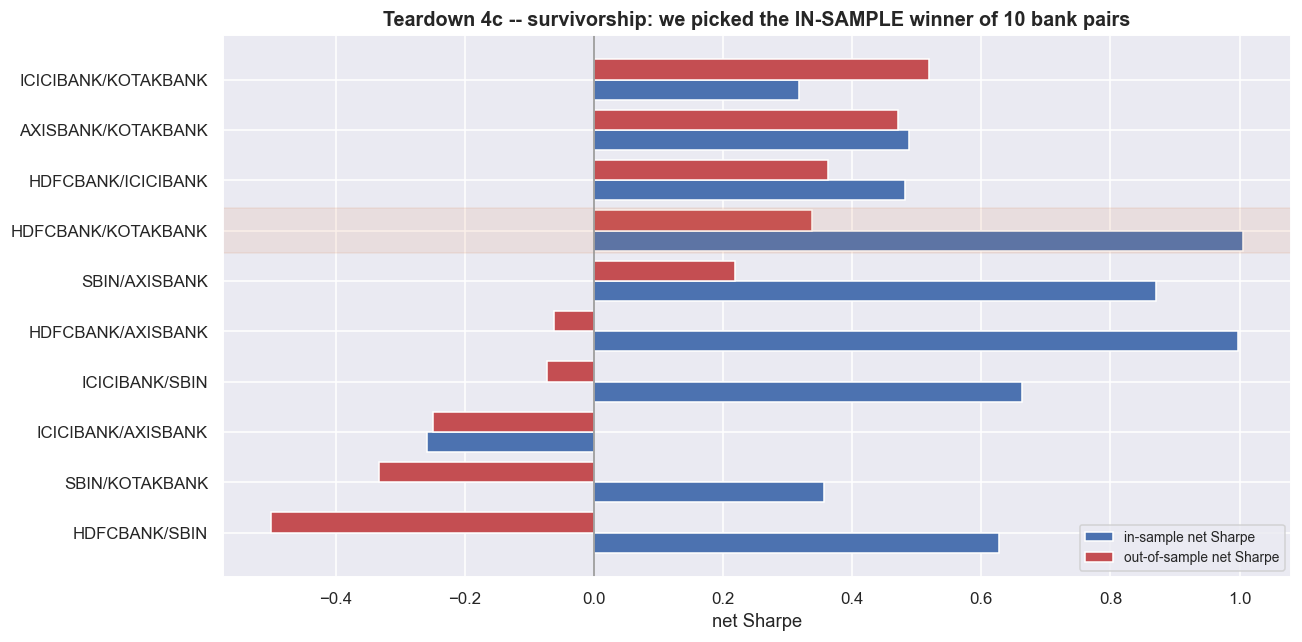
Our pair ranked first of ten in-sample. Run the identical net strategy across all ten same-sector bank pairs, and 5 of the 10 actually lose money net out of sample. We did not so much find a good pair as run a beauty contest in-sample and crown a winner. That crown is worth little once the window changes. And these are only the banks still in the index. The pairs that merged or delisted are not on the chart at all. So even this humbling picture is the flattering version.
A low p-value pulled from a scan of many pairs is a hypothesis, not a discovery. Scan ten pairs, and the best one looks special just by construction. Scan a hundred, and a few will pass any test by chance alone. The honest number is not the winner's in-sample Sharpe. It is how the whole group - winners, losers, and the delisted ghosts - did out of sample.
The honest verdict
Put every view of the same strategy side by side and the story is plain. The seductive in-sample net Sharpe of 1.01 is the best case. Every honest adjustment moves it toward zero.
| View | Sharpe | Ann. vol | Total | Max DD |
|---|---|---|---|---|
| In-sample gross | 1.14 | 16.4% | +134.2% | -20.5% |
| In-sample net | 1.01 | 16.4% | +110.5% | -20.9% |
| Out-of-sample gross | 0.46 | 17.8% | +17.5% | -13.8% |
| Out-of-sample net | 0.34 | 17.8% | +11.5% | -13.8% |
| Walk-forward 2024+ net | 0.62 | 15.1% | +22.3% | -13.3% |
And here is the chart we are not allowed to hide - the one a brochure would crop out.
# The chart you are not allowed to hide: the honest, net, out-of-sample equity curve.
no  = eqc(bt['net'].loc[ooS]); p = perf(bt['net'].loc[ooS])
dd  = no/no.cummax() - 1
fig, (ax1, ax2) = plt.subplots(2, 1, figsize=(12, 6.6), sharex=True,
                               gridspec_kw=dict(height_ratios=[3, 1]))
ax1.plot(no.index, no.values, color=C['red'], lw=2.2)
ax1.axhline(1, color=C['grey'], lw=1.0, ls='--')
ax1.fill_between(no.index, 1, no.values, where=(no.values>=1), color=C['green'], alpha=0.10)
ax1.fill_between(no.index, 1, no.values, where=(no.values< 1), color=C['red'],   alpha=0.10)
ax1.set_ylabel('growth of Rs 1')
ax1.set_title(f'The honest bottom line: NET, OUT-OF-SAMPLE equity  ({A_name}/{B_name})\n'
              f'Sharpe {p["sharpe"]:.2f}   total {p["total"]*100:+.1f}%   max drawdown {p["maxdd"]*100:.1f}%')
ax2.fill_between(dd.index, dd.values*100, 0, color=C['red'], alpha=0.35)
ax2.set_ylabel('drawdown (%)'); ax2.set_xlabel('')
plt.tight_layout(); plt.show()

print(f'Net of realistic NSE costs, out of sample, over {(pd.Timestamp(OO1)-pd.Timestamp(OO0)).days/365.25:.1f} years,')
print(f'this much-celebrated pair returned {p["total"]*100:+.1f}% at a Sharpe of {p["sharpe"]:.2f} -- before a single')
print(f'rupee of borrow cost, financing, slippage beyond our estimate, or the equity-short problem. That is the truth.')Net of realistic NSE costs, out of sample, over 2.5 years, this much-celebrated pair returned +11.5% at a Sharpe of 0.34 -- before a single rupee of borrow cost, financing, slippage beyond our estimate, or the equity-short problem. That is the truth.
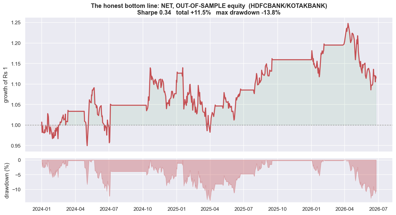
This is the net, out-of-sample equity curve, drawdowns and all. It is the only curve that matches money you could actually have kept. Over two and a half years it returned +11.5% at a Sharpe of 0.34. And even that is before a single rupee of borrow cost, financing, slippage beyond our estimate, or the plain fact that you cannot freely hold a short equity position for weeks. An honest researcher publishes this curve, not the seductive one at the top.
Where this breaks
The strategy did not fail because of a bug. It failed because a backtest measures how well a rule fit the past, while trading needs how well a rule survives the future. The gap between those two is everything we just measured.
- The in-sample curve was a hypothesis. Tested on fresh data, the net Sharpe fell from 1.01 to 0.34 in this window. Re-fitting the hedge ratio recovers part of that, to 0.62, but still lands far below the headline and adds its own overfitting risk.
- Costs are not a footnote. Eight fills per round trip, dominated by delivery transaction tax, turned a comfortable gross 0.90 into a marginal net 0.77. And the out-of-sample result flips from profit to loss somewhere around a 1.9% round-trip cost you cannot pin down in advance.
- The relationship was never stable. The pair failed the cointegration test in about 90% of rolling windows, and the hedge ratio swung 317% of its mean, even going negative. A fixed spread trades a relationship that has already ended.
- Leaks flatter quietly. A one-day shift in the fill, or a full-sample normalisation, moved the result by more than the entire edge, in either direction. And we crowned the in-sample winner of ten survivors while the broken and delisted pairs stayed invisible.
The bottom line: naive pairs trading on HDFCBANK / KOTAKBANK, net of realistic NSE costs and out of sample, is at best marginal. That means a low single-digit Sharpe and a near-flat equity curve - and that is before borrow, financing, slippage beyond our estimate, and the short-leg problem. A statistical relationship existed in one window. That is genuinely not the same thing as a tradable edge. The difference between the two is the price of admission to everything that follows. This is not a counsel of despair. It is the standard every later technique must clear before it earns a place in the book: dynamic hedge ratios, baskets, cross-sectional neutrality, proper sizing, and validation that does not fool you. Every one of them has to pass the same four leaks measured here. Educational content only, not investment advice.