Finding Pairs Without Fooling Yourself
Economic prior first, then the cointegration scan, then the multiple-testing trap: scanning many pairs guarantees false positives. Bonferroni and false-discovery control, and how few survive out-of-sample.
- ·Economic prior first
- ·The cointegration scan
- ·The multiple-testing trap
- ·False positives in random data
- ·Bonferroni and FDR control
- ·How few survive
A cointegration p-value of 0.03 feels like a discovery. Cointegration means two prices that each wander on their own are still tied together, so a combination of them keeps reverting to an average. The p-value is the chance, if the two really were unrelated, of seeing a result at least this extreme; below 0.05 counts as evidence (it is not the probability that they are unrelated). Run the test once, on a pair you had a genuine economic reason to test, and a low p-value is a real signal. Run it across five hundred pairs and keep the ones below 0.05, and you have not built a watchlist - you have built a machine for manufacturing false positives. The test never changed. The number of tests did. That problem is called multiple testing, and it is the subject of this chapter: how to search a whole universe for tradable pairs without fooling yourself along the way. The punchline on real NSE data over this window is bleak. A disciplined funnel that starts with 73 candidate pairs ends with zero that survive every honest gate. Far better to learn why here than to pay for the lesson with a trading account.
Start with a reason, not a scan
The original sin of pairs research is the blind scan. Our universe here is 50 NSE names. With 50 names there are C(50, 2) = 1,225 possible pairs. Point a cointegration test at all of them, keep everything under p < 0.05, and pure chance alone hands you roughly 0.05 x 1,225 = 61 "cointegrated" pairs that mean absolutely nothing. Worse, you have no way to tell those 61 ghosts apart from anything real. You have not screened a universe. You have bought 1,225 lottery tickets and circled the winners after the draw.
The fix is an economic prior: only test pairs that have a structural reason to share a long-run driver. Two private banks, two IT-services exporters, two steelmakers - names exposed to the same demand, the same input costs, the same regulation and rate cycle - are at least plausibly tethered. Restricting the scan to within-sector pairs is not just good economics. It is good statistics, because it cuts the number of tests from 1,225 to 78 same-sector candidates (6.4% of the blind universe). That single decision drops the expected pure-chance "winners" from about 61 to about 4. Nothing else in this chapter moves the false-discovery problem as hard as choosing what not to test.
from math import comb
import itertools

# Load the price panel once from the cached DuckDB.
px = closes(UNIVERSE, start="2016-01-01", end="2026-06-26")
print("panel:", px.shape, "|", px.index.min().date(), "->", px.index.max().date())

# Stage 1: candidate pairs come ONLY from within a sector (the economic prior).
CAND = []
for sec, names in SECTORS.items():
    names = [s for s in names if s in px.columns]
    for a, b in itertools.combinations(names, 2):
        CAND.append((a, b))

per_sector = pd.Series({sec: comb(len([s for s in names if s in px.columns]), 2)
                        for sec, names in SECTORS.items()})
per_sector = per_sector[per_sector > 0].sort_values(ascending=False)

full_universe = comb(px.shape[1], 2)
print(f"Blind scan would test C({px.shape[1]},2) = {full_universe} pairs.")
print(f"Same-sector prior tests only {len(CAND)} pairs "
      f"({100*len(CAND)/full_universe:.1f}% of the blind universe).")
print(f"At p<0.05, expected pure-chance 'winners':  blind ~ {0.05*full_universe:.0f},  "
      f"prior ~ {0.05*len(CAND):.0f}.")

fig, ax = plt.subplots(figsize=(11, 4.8))
sns.barplot(x=per_sector.values, y=per_sector.index, hue=per_sector.index,
            palette="crest", legend=False, ax=ax)
for i, v in enumerate(per_sector.values):
    ax.text(v + 0.1, i, str(int(v)), va="center", fontsize=9)
ax.set_title(f"Same-sector candidate pairs per sector  (total = {len(CAND)})")
ax.set_xlabel("number of within-sector pairs"); ax.set_ylabel("")
plt.tight_layout(); plt.show()panel: (3195, 50) | 2016-01-01 -> 2026-06-25 Blind scan would test C(50,2) = 1225 pairs. Same-sector prior tests only 78 pairs (6.4% of the blind universe). At p<0.05, expected pure-chance 'winners': blind ~ 61, prior ~ 4.
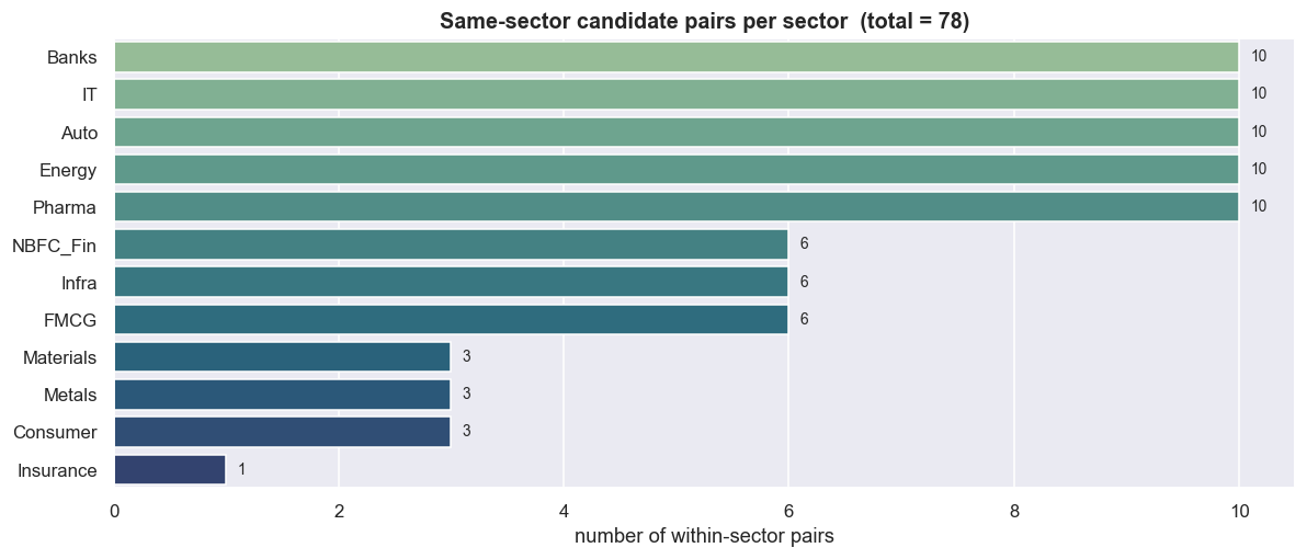
The biggest lever on false discovery is not the correction you apply at the end. It is the size of the search you start with. A same-sector prior shrinks the test count roughly 16-fold (1,225 -> 78) and the expected pure-chance winners from ~61 to ~4 before a single test runs. Choosing what not to test is the cheapest risk control in the field.
The scan: 16 of 73 "pass"
Two honesty rules go in before any scan. First, the scan and the verdict use different data. We split time into two parts. The in-sample window (2018-01-01 to 2023-12-31) is the data we scan and correct on - the data we are allowed to mine. The out-of-sample window (2024-01-01 to today) is fresh data the scan never touches, held back as the only honest test. If a pair only looks tethered because we peeked at its whole history, the held-back window will catch it. Second, thin histories are dropped, not stretched. Recent listings and renames lack a full in-sample window, and a cointegration test on a short overlap is just noise, so we require a minimum number of in-sample rows. That requirement drops 5 of the 78 candidates, leaving 73 pairs with enough history to test.
The test itself is Engle-Granger on log price levels. Its null hypothesis is no cointegration, so a small p-value is evidence the pair is tethered. Run it across all 73 pairs and the heatmap below shows the result sector by sector - the colour is reversed, so bright cells are the low p-values.
def sector_pmatrix(names):
    names = [s for s in names if s in px.columns]
    M = pd.DataFrame(np.nan, index=names, columns=names)
    for a, b in itertools.combinations(names, 2):
        p, n = coint_p(a, b, *IS)
        if n >= MIN_IS:
            M.loc[a, b] = M.loc[b, a] = p
    np.fill_diagonal(M.values, 0.0)
    return M

show = ["Banks", "IT", "Energy", "Auto", "Pharma", "NBFC_Fin"]
fig, axes = plt.subplots(2, 3, figsize=(15, 9))
for ax, sec in zip(axes.ravel(), show):
    M = sector_pmatrix(SECTORS[sec])
    mask = np.triu(np.ones_like(M, dtype=bool), k=1)
    sns.heatmap(M, mask=mask, ax=ax, cmap="rocket_r", vmin=0, vmax=1,
                annot=True, fmt=".2f", annot_kws={"size": 8}, cbar=False,
                linewidths=.5, linecolor="#0d1117")
    ax.set_title(f"{sec}  (bright = coint, p<0.05)", fontsize=11)
    ax.set_xticklabels(ax.get_xticklabels(), rotation=45, ha="right", fontsize=8)
    ax.set_yticklabels(ax.get_yticklabels(), rotation=0, fontsize=8)
plt.suptitle("In-sample cointegration p-values within each sector", y=1.01,
             fontsize=13, fontweight="bold")
plt.tight_layout(); plt.show()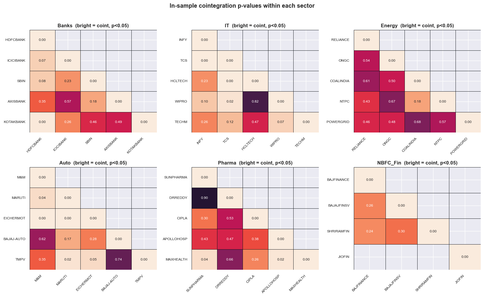
Notice how few cells light up, even within a sector. Belonging to the same industry buys you a sensible hypothesis. It never buys you a guaranteed tether. Keep every pair with p < 0.05 and the naive scan hands you 16 of the 73 as "cointegrated." Sixteen pairs. That is what an undisciplined screen would print, frame as a watchlist, and start trading. Hold that number in your head, because the next stage asks the only question that matters: how many of those 16 would you have found in pure noise?
How many would pure noise hand you?
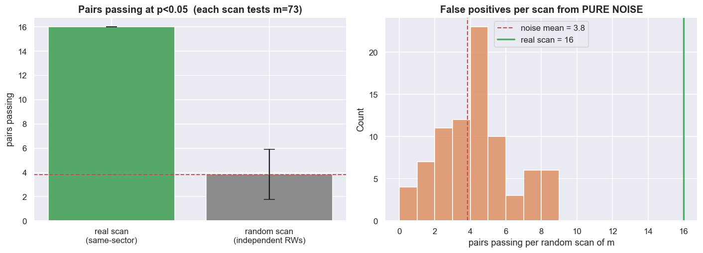
Here is the uncomfortable experiment. Build the same number of independent random-walk pairs we just tested. A random walk is a price whose next value is just today's value plus random noise, so two of them have no relationship whatsoever. Scan those for cointegration anyway. Because the Engle-Granger test is set to a 5% significance level, roughly 5% of these noise pairs will "pass" at p < 0.05 by sheer luck. We drew 6,000 independent random-walk pairs (seeded, each of length T = 1,484 to match the typical in-sample size) and measured the false-positive rate directly: 5.25%, almost exactly the 5% the test promises. Multiply that by our 73 tests and the expected number of fake "cointegrated" pairs from pure noise is about 3.8.
So the real scan found 16. Roughly 4 of those are what a scan of this size would have thrown up from nothing, leaving about 12 above the noise floor. That gap, not the raw count of 16, is the only part that could be real. Put bluntly: a quarter of the watchlist a naive screen just handed you is statistically indistinguishable from coin flips. The chart below puts the real scan beside the full spread of false positives from pure noise.
rng = np.random.default_rng(20260629)
K   = 6000                                   # pool of independent random-walk pairs
T   = int(scan.n_is.median())                # match the typical in-sample length
pmc = np.empty(K)
for i in range(K):
    x = np.cumsum(rng.standard_normal(T))    # random walk 1
    y = np.cumsum(rng.standard_normal(T))    # random walk 2 - totally unrelated
    pmc[i] = cp(x, y)

rate         = (pmc < 0.05).mean()
R            = K // m
blocks       = pmc[:R * m].reshape(R, m)
block_counts = (blocks < 0.05).sum(axis=1)   # passes per random scan of size m
exp_random   = rate * m
n_naive      = len(naive)

fig, ax = plt.subplots(1, 2, figsize=(13, 4.8))
ax[0].bar(["real scan\n(same-sector)", "random scan\n(independent RWs)"],
          [n_naive, block_counts.mean()],
          yerr=[0, block_counts.std()], capsize=7,
          color=[C["green"], C["grey"]])
ax[0].axhline(exp_random, color=C["red"], ls="--", lw=1.3)
ax[0].set_title(f"Pairs passing at p<0.05  (each scan tests m={m})")
ax[0].set_ylabel("pairs passing")
sns.histplot(block_counts, bins=range(0, int(block_counts.max()) + 2),
             color=C["amber"], ax=ax[1])
ax[1].axvline(exp_random, color=C["red"], ls="--", lw=1.4,
              label=f"noise mean = {exp_random:.1f}")
ax[1].axvline(n_naive, color=C["green"], lw=2.2, label=f"real scan = {n_naive}")
ax[1].set_title("False positives per scan from PURE NOISE")
ax[1].set_xlabel("pairs passing per random scan of m"); ax[1].legend()
plt.tight_layout(); plt.show()

print(f"Monte Carlo: {K} independent random-walk pairs (length T={T}), seed=20260629.")
print(f"  False-positive RATE at p<0.05 = {rate*100:.2f}%   (the test's size; nominal 5%).")
print(f"  Expected spurious 'cointegrated' pairs in a scan of m={m}: {exp_random:.1f}.")
print(f"  Real same-sector scan found {n_naive}  ->  about {max(n_naive-exp_random,0):.1f} above the noise floor.")
print("So a chunk of the naive winners are statistically indistinguishable from coin flips.")Monte Carlo: 6000 independent random-walk pairs (length T=1484), seed=20260629. False-positive RATE at p<0.05 = 5.25% (the test's size; nominal 5%). Expected spurious 'cointegrated' pairs in a scan of m=73: 3.8. Real same-sector scan found 16 -> about 12.2 above the noise floor. So a chunk of the naive winners are statistically indistinguishable from coin flips.
A low p-value pulled from a large scan is a hypothesis, not a discovery. At a 5% threshold the test is designed to fire on about one in twenty unrelated pairs, so the more pairs you test, the more meaningless passes you collect. Never quote a single pair's p-value without also saying how many pairs you tested to find it. The winner's p-value only means something once you know the size of the search.
Clawing it back: Bonferroni and BH-FDR
Two standard corrections turn "I ran one test" maths into "I ran 73 tests" maths. They trade off boldness against safety very differently.
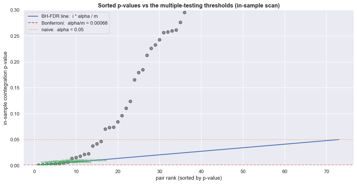
Bonferroni controls the chance of even one false positive across the whole batch of tests. The rule is brutally simple: only believe a pair whose p-value is below alpha / m, here 0.05 / 73 = 0.00068. With dozens of tests that threshold is tiny, so Bonferroni is cautious by design - it will throw out genuine pairs to be sure it admits no junk. In this window exactly 1 of the 16 survives it.
Benjamini-Hochberg (BH) FDR is gentler. Instead of forbidding every false positive, it controls the expected fraction of false discoveries among the pairs you keep. Sort the p-values from smallest to largest. The largest rank i where p(i) <= (i / m) x alpha sets the cutoff, and you keep everything at or below it. BH keeps more pairs than Bonferroni while still capping the junk rate. Here the cutoff lands at p <= 0.0048 and 7 pairs survive.
alpha   = 0.05
p       = scan.p_is.values
order   = np.argsort(p)
ps      = p[order]
names_s = scan.pair.values[order]
ranks   = np.arange(1, m + 1)

bonf_thr = alpha / m
bh_line  = alpha * ranks / m
passed   = ps <= bh_line
bh_cut   = ps[passed].max() if passed.any() else -np.inf

n_bonf = int((p < bonf_thr).sum())
n_bh   = int((p <= bh_cut).sum())

fig, ax = plt.subplots(figsize=(11.5, 6))
dot_col = [C["green"] if v <= bh_cut else C["grey"] for v in ps]
ax.scatter(ranks, ps, s=48, color=dot_col, zorder=3, edgecolor="#0d1117", linewidth=.5)
ax.plot(ranks, bh_line, color=C["blue"], lw=1.9, label="BH-FDR line:  i * alpha / m")
ax.axhline(bonf_thr, color=C["red"], ls="--", lw=1.6, label=f"Bonferroni:  alpha/m = {bonf_thr:.5f}")
ax.axhline(alpha, color=C["amber"], ls=":", lw=1.4, label="naive:  alpha = 0.05")
for rk, (pp, nm) in enumerate(zip(ps, names_s), start=1):
    if pp <= bh_cut:
        ax.annotate(nm, (rk, pp), fontsize=8, color=C["green"],
                    xytext=(5, 4), textcoords="offset points")
ax.set_ylim(0, 0.30); ax.set_xlabel("pair rank (sorted by p-value)")
ax.set_ylabel("in-sample cointegration p-value")
ax.set_title("Sorted p-values vs the multiple-testing thresholds (in-sample scan)")
ax.legend(loc="upper left")
plt.tight_layout(); plt.show()

bh_disp = bh_cut if np.isfinite(bh_cut) else float("nan")
print(f"m = {m} same-sector tests on the common in-sample window.")
print(f"  Naive     (p<0.05)          : {n_naive} pairs")
print(f"  Bonferroni (p<{bonf_thr:.5f})    : {n_bonf} pairs survive")
print(f"  BH-FDR    (q=0.05, cut p<={bh_disp:.4f}): {n_bh} pairs survive")
print("Notice how many 'winners' were really just the cost of running a big scan.")m = 73 same-sector tests on the common in-sample window. Naive (p<0.05) : 16 pairs Bonferroni (p<0.00068) : 1 pairs survive BH-FDR (q=0.05, cut p<=0.0048): 7 pairs survive Notice how many 'winners' were really just the cost of running a big scan.
Bonferroni answers "how do I avoid any false positive?" BH answers "how do I keep the false-positive fraction small while still finding things?" Neither is universally right. Bonferroni suits a setting where one bad pair is catastrophic. BH suits a research pipeline where a controlled minority of duds is acceptable, because every survivor still faces a further out-of-sample gate. We use BH precisely because that next gate exists.
The arithmetic is sobering on its own. Of the 16 pairs the naive screen called discoveries, 9 were demoted the moment we accounted for having run 73 tests rather than one. They were never findings. They were the price of the scan.
The only referee that counts: out-of-sample
Everything so far happened on the in-sample window - the data we mined. A pair that survives correction in-sample is, at best, a strong hypothesis. It is not a result, because we chose the window, the universe and the sector map specifically to surface it. The honest referee is data the scan never saw. So we re-run cointegration on the held-back 2024-to-today window and keep only the pairs that hold up there too.
Brace for it. Of the 7 BH-FDR survivors, the number that stay cointegrated at p < 0.05 on the out-of-sample window is zero. Not one. The funnel that began with 73 candidates, narrowed to 16, and was corrected down to 7, collapses to 0 out-of-sample-confirmed pairs in this window. The disciplined search, run honestly end to end, finds nothing it can stand behind.
stages = ["Candidate\nsame-sector pairs", "Naive  p<0.05",
          "BH-FDR survivors", "OOS-confirmed"]
counts = [m, n_naive, n_bh, n_final]
ypos   = np.arange(len(stages))[::-1]
cols   = [C["grey"], C["amber"], C["blue"], C["green"]]

fig, ax = plt.subplots(figsize=(10.5, 5))
ax.barh(ypos, counts, color=cols, height=0.62)
for y, c in zip(ypos, counts):
    ax.text(c + max(counts) * 0.012, y, str(c), va="center", fontweight="bold")
ax.set_yticks(ypos); ax.set_yticklabels(stages)
ax.set_xlabel("pairs surviving"); ax.set_xlim(0, max(counts) * 1.12)
ax.set_title("The honest funnel: prior -> test -> correct -> confirm OOS (this window)")
plt.tight_layout(); plt.show()

print("Survivors of the full disciplined pipeline (BH-FDR AND out-of-sample):")
final = bh_oos[bh_oos.holds_oos][["pair", "sector", "p_is", "p_oos"]]
if len(final):
    display(final.reset_index(drop=True))
else:
    print("  NONE this window: nothing that survives correction also confirms out-of-sample.")
print(f"\nStage counts (live): candidates={m}, naive={n_naive}, "
      f"Bonferroni={n_bonf}, BH-FDR={n_bh}, OOS-confirmed={n_final}.")
print("On a different in-sample/out-of-sample split these counts change - that fragility is the lesson.")Survivors of the full disciplined pipeline (BH-FDR AND out-of-sample): NONE this window: nothing that survives correction also confirms out-of-sample. Stage counts (live): candidates=73, naive=16, Bonferroni=1, BH-FDR=7, OOS-confirmed=0. On a different in-sample/out-of-sample split these counts change - that fragility is the lesson.
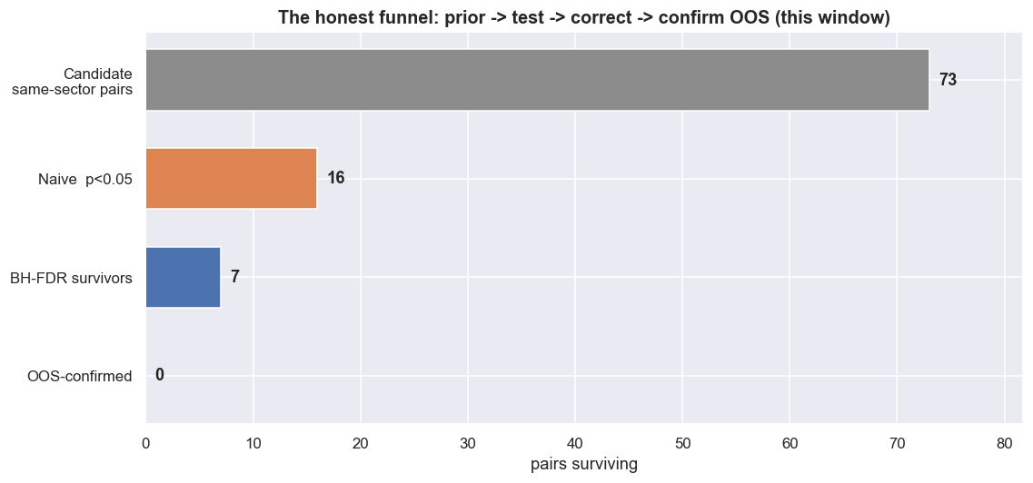
That zero is not a bug in the method. It is the method working. The whole apparatus - the prior, the noise simulation, the two corrections, the held-back window - exists to make exactly this outcome visible before capital is committed, not after. An undisciplined screen would have stopped at the 16-pair bar, declared victory, and traded a watchlist with about 4 pure-noise pairs baked in and no out-of-sample evidence for any of them.
Fix every rule of the search - window, universe, sector map, minimum history, correction, out-of-sample split - before you look at a single result. Then report the entire funnel, not just the bottom bar. The corrections control error given the tests you ran. They cannot undo a search that was redesigned until it produced winners. "Zero survivors this window" is a legitimate, publishable answer. Forcing a non-zero answer is how the fooling starts.
The honest workflow
Compress the chapter to one line and it reads: economic prior -> scan on a common in-sample window -> correct for multiple testing -> confirm out-of-sample -> only then consider costs and tradability.
Skip the prior and you scan 1,225 pairs and drown in roughly 61 false positives. Skip the correction and you trade noise that "passed" at p < 0.05 only because you ran 73 tests. Skip out-of-sample and you trade a relationship you fitted to history and never challenged. Each gate exists because the gate before it is not enough. And a pair that clears all four is still only a candidate - it has earned the right to be cost-tested, nothing more. The exact numbers will differ on a different window, but the shape never does. The funnel always narrows, usually far more brutally than the top bar promised.
Check yourself
1. You test 73 pairs at the 5% level. Roughly how many false positives do you expect from luck alone?
About 73 x 0.05, so three or four "significant" pairs even if none are truly cointegrated. That is why a raw scan of low p-values is a false-positive machine.
2. What does the Bonferroni correction control, and what does it cost you?
It controls the chance of even one false positive across the whole batch, by demanding a p-value below alpha/m (here 0.05/73 = 0.00068). The cost is power: it is so strict it throws out genuine pairs to be sure it admits no junk.
3. The honest funnel ended with zero surviving pairs. Is that a failure of the method?
No - it is the method working. Finding nothing tradable in this window, after multiple-testing discipline and out-of-sample checks, is a far cheaper lesson than trading a false positive. An honest "no" is a result.
Where this breaks
- Selection bias dwarfs the p-value. Even after Bonferroni and BH, the pairs you keep are the best of a search you designed. The corrections control error given the set of tests you ran - not the human choices that built that set: the window, the universe, the sector map, the minimum-history cut. Tweak any of those and a different set of "survivors" appears. The only defence is fixing the rules before you look, and reporting the whole funnel.
- The universe is a survivor-only set. These are today's index members. Names that were dropped, merged or delisted never enter the scan, which flatters every survival rate here. A true point-in-time universe that still carried its dead names would push the hit rate lower.
- One out-of-sample window is one draw. A single 2024-to-today window is a single referee. A pair can confirm here and die next quarter, or fail here on a two-year wobble and be perfectly tethered over a decade. One out-of-sample pass is evidence, not proof. Walk-forward testing repeats this check many times, and the survival rate keeps falling.
- The corrections assume the tests are roughly independent. Same-sector pairs share legs - one bank name appears in several bank pairs - so the p-values are correlated. Bonferroni is then too harsh, and BH's guarantee becomes approximate. The direction of the lesson holds, but the exact survivor count is softer than the clean integers suggest.
- A surviving tether is still not an edge. Nothing here touched the bid-ask spread, the transaction costs, the short-leg vehicle, the half-life, or the capacity. Passing this funnel only earns a pair the right to be cost-tested. In Indian markets the short leg needs a real vehicle - an intraday cash short, a borrowed-stock arrangement, or a stock-futures proxy - each with its own cost, margin and availability. Finding a pair without fooling yourself is the cheap part. Everything the rest of this course adds on top is the expensive part.