Capital Allocation & Sizing

You have a real edge and a diversified portfolio. One question remains, and it decides whether you compound a fortune or go broke anyway: how much do you bet? This is sizing at the portfolio level - not "how many shares of this stock" (that was the /python course) but "how much of my total capital does each position and each strategy deserve?" Bet too little and a good edge barely grows your wealth; bet too much and the same edge destroys you. There is a mathematically optimal answer, and the cliff right next to it is the most important thing in this chapter.

The Kelly criterion

In 1956 a Bell Labs physicist, John Kelly, derived the bet size that maximises the long-run growth rate of your capital. For a return stream, it's roughly your edge divided by your variance - and betting more than that doesn't grow you faster, it grows you slower and eventually ruins you. Let's see the entire curve on real Nifty data:

# The Kelly criterion: the bet size that maximises long-run growth - and the cliff beyond it.
import os
from datetime import datetime

from openalgo import api

client = api(
    api_key=os.getenv("OPENALGO_API_KEY", "your_api_key_here"),
    host=os.getenv("OPENALGO_HOST", "http://127.0.0.1:5000"),
)

end = datetime.now().strftime("%Y-%m-%d")
r = client.history(symbol="NIFTY", exchange="NSE_INDEX", interval="D",
                   start_date="2021-01-01", end_date=end)["close"].pct_change().dropna()

# For a return stream, the growth-optimal (Kelly) leverage is roughly mean / variance.
kelly_lev = r.mean() / r.var()
print(f"Nifty daily edge: mean {r.mean() * 100:.3f}%, vol {r.std() * 100:.2f}%")
print(f"Growth-optimal (full Kelly) leverage: {kelly_lev:.1f}x\n")

print(f"{'BET SIZE':>16s}{'FINAL WEALTH (x)':>18s}")
for mult in [0.25, 0.5, 1.0, 1.5, 2.0, 3.0]:
    final = (1 + kelly_lev * mult * r).prod()
    label = {0.5: " (half Kelly)", 1.0: " (full Kelly)"}.get(mult, "")
    print(f"{str(round(mult, 2)) + 'x Kelly' + label:>16s}{final:>18.2f}")

print("\nGrowth peaks near FULL Kelly, then collapses - over-betting destroys wealth even with an edge.")

Nifty daily edge: mean 0.044%, vol 0.90%
Growth-optimal (full Kelly) leverage: 5.4x

        BET SIZE  FINAL WEALTH (x)
     0.25x Kelly              2.02
0.5x Kelly (half Kelly)              3.33
1.0x Kelly (full Kelly)              4.87
      1.5x Kelly              2.99
      2.0x Kelly              0.71
      3.0x Kelly              0.00

Growth peaks near FULL Kelly, then collapses - over-betting destroys wealth even with an edge.

Read the numbers against the curve. Quarter-Kelly multiplied wealth ~2x; half-Kelly ~3.3x; full Kelly ~4.9x - the peak. Then it reverses: 1.5x Kelly drops to ~3x, 2x Kelly actually loses money (0.7x), and 3x Kelly is total ruin. This is the lesson that humbles every aggressive trader: past the optimum, betting more with a winning edge makes you poorer. The cliff is right there, just beyond the peak.

Why full Kelly is still too aggressive

Even the peak is dangerous in practice, for two reasons. First, full Kelly is brutally volatile - it maximises growth but accepts gut-wrenching drawdowns of 50% or more along the way, which no human (or investor) actually tolerates. Second, Kelly assumes you know your edge exactly - and you don't (Chapter 13). Over-estimate your edge and your "full Kelly" is really 2x or 3x Kelly - straight off the cliff.

Fractional Kelly

So professionals bet a fraction of Kelly - typically a half or a quarter. Look back at the table: half-Kelly captured most of the growth (3.3x of the 4.9x peak) with far less volatility and a huge safety margin against over-estimating your edge. Fractional Kelly is the sane default: most of the upside, a fraction of the risk, and protection against your own optimism.

Volatility targeting

Kelly tells you the size; volatility targeting keeps that size honest as markets change. Pick a target risk level (say 12% annualised) and scale your exposure inversely to recent volatility - smaller when the market is wild, larger when it's calm - so your risk stays roughly constant even as conditions swing:

Copy

# Volatility targeting: scale exposure so risk stays steady - down in storms, up in calm.
import os
from datetime import datetime
from pathlib import Path

import matplotlib

matplotlib.use("Agg")
import matplotlib.pyplot as plt
import seaborn as sns
from openalgo import api

client = api(
    api_key=os.getenv("OPENALGO_API_KEY", "your_api_key_here"),
    host=os.getenv("OPENALGO_HOST", "http://127.0.0.1:5000"),
)

end = datetime.now().strftime("%Y-%m-%d")
df = client.history(symbol="NIFTY", exchange="NSE_INDEX", interval="D",
                    start_date="2021-01-01", end_date=end)
r = df["close"].pct_change()

TARGET = 12.0                                            # target annualised volatility, %
realized = r.rolling(20).std() * (252 ** 0.5) * 100      # recent realised vol
exposure = (TARGET / realized).clip(upper=2.5)           # scale, capped at 2.5x leverage
exposure = exposure.dropna()

sns.set_theme(style="whitegrid")
fig, ax = plt.subplots(figsize=(8, 4.5))
ax.plot(exposure.index, exposure, color="#7c83ff", lw=1.4)
ax.axhline(1.0, color="#888", ls="--", lw=1, label="full exposure")
ax.fill_between(exposure.index, exposure, 1.0, where=exposure < 1, color="#dc2626", alpha=0.18)
ax.fill_between(exposure.index, exposure, 1.0, where=exposure > 1, color="#16a34a", alpha=0.18)
ax.set_title(f"Volatility targeting ({TARGET:.0f}% target) - exposure shrinks in turbulent times")
ax.set_ylabel("Position size (x capital)")
ax.legend()

out = Path(__file__).with_suffix(".png")
plt.savefig(out, dpi=110, bbox_inches="tight")
print(f"Exposure ranges {exposure.min():.2f}x (storms) to {exposure.max():.2f}x (calm), now {exposure.iloc[-1]:.2f}x. Saved {out.name}")

Live output

Exposure ranges 0.40x (storms) to 2.39x (calm), now 0.93x. Saved 02_vol_targeting.png

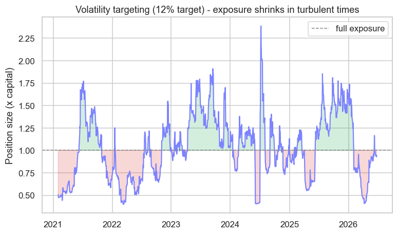
Watch the exposure breathe: it drops below 0.5x in turbulent stretches and climbs above 2x in calm ones, all to hold risk steady. This is one of the most robust ideas in allocation - it automatically pulls you out of harm's way exactly when volatility (and danger) spikes, the early-warning value of the GARCH forecasts from Chapter 16.

Risk parity

The same principle scales to a whole book. Risk parity allocates so that each asset or strategy contributes equal risk - not equal capital. A volatile holding gets a smaller rupee weight, a calm one a larger weight, so no single position dominates the portfolio's swings. It's the antidote to the hidden trap of equal-capital weighting, where your most volatile holding quietly drives almost all the risk.

Allocating across strategies

At the top level, you're not sizing trades - you're sizing strategies. Combine several genuinely uncorrelated edges (a trend-follower, a mean-reverter, a vol-seller), size each by its risk contribution, cap the total, and rebalance. For blending your own views with the market's, Black-Litterman offers a robust alternative to raw mean-variance: it starts from the market's equilibrium weights and tilts gently toward your views in proportion to your confidence - sidestepping the error-maximisation of Chapter 23.

Try it yourself

• Compute Kelly for a single stock with a stronger edge than the index. Is its optimal leverage higher or lower, and how brutal is the over-betting cliff?
• Backtest the volatility-targeted Nifty exposure against a constant 1x. Does targeting improve the Sharpe ratio and shrink the worst drawdown?
• Build a two-strategy risk-parity weight: given two strategies' volatilities, what weights make their risk contributions equal? (Hint: inverse-volatility.)

Recap

• Sizing decides survival: even a winning edge is destroyed by over-betting.
• The Kelly criterion is the growth-optimal bet size - but growth peaks there and collapses beyond (full Kelly ~4.9x, 2x Kelly lost money, 3x was ruin).
• Full Kelly is too aggressive in practice - hugely volatile and fatally sensitive to over-estimating your edge - so professionals bet fractional Kelly (a half or quarter).
• Volatility targeting scales exposure inversely to risk, holding portfolio volatility steady and pulling you out of storms automatically.
• Risk parity equalises risk (not capital) across positions, and at the book level you size strategies by risk, blending views robustly with Black-Litterman.

We've sized for the normal world. But markets have a fat-tailed abnormal world (Chapter 11), and that's where accounts die. The final chapter of this module faces it head-on: tail risk, Value-at-Risk, expected shortfall, and stress testing.