Returns & the Stylized Facts

We've spent ten chapters on how the market works. Now we pick up the quant's other toolkit: the mathematics that lets us model it. And the very first thing to model is the return itself - the percentage change that is the atom of everything we do. Returns seem boring and simple. They are not. They have a distinct, stubborn personality - a set of patterns so universal that academics named them the stylized facts of returns - and that personality quietly breaks half of classical finance. Meet your raw material properly.

Simple versus log returns

There are two ways to measure a return, and the difference matters more than it looks:

# Two ways to measure a return - and why quants quietly prefer logs.
import os
from datetime import datetime, timedelta

import numpy as np
from openalgo import api

client = api(
    api_key=os.getenv("OPENALGO_API_KEY", "your_api_key_here"),
    host=os.getenv("OPENALGO_HOST", "http://127.0.0.1:5000"),
)

end = datetime.now().strftime("%Y-%m-%d")
start = (datetime.now() - timedelta(days=365)).strftime("%Y-%m-%d")
p = client.history(symbol="NIFTY", exchange="NSE_INDEX", interval="D",
                   start_date=start, end_date=end)["close"]

simple = p.pct_change().dropna()
logret = np.log(p / p.shift(1)).dropna()

print("Last 5 simple returns:", [round(x, 5) for x in simple.tail(5)])
print("Last 5 log returns   :", [round(x, 5) for x in logret.tail(5)])
print("(almost identical for small daily moves)\n")

# The magic of logs: they ADD across time.
print(f"Sum of daily log returns : {logret.sum():.5f}")
print(f"Log of the whole move    : {np.log(p.iloc[-1] / p.iloc[0]):.5f}   <- matches exactly")
print(f"Sum of simple returns    : {simple.sum():.5f}")
print(f"Actual compounded return : {(1 + simple).prod() - 1:.5f}   <- simple returns do NOT add")

Last 5 simple returns: [0.00342, -0.00641, 0.00374, -0.01157, 0.00829]
Last 5 log returns   : [0.00341, -0.00643, 0.00373, -0.01163, 0.00826]
(almost identical for small daily moves)

Sum of daily log returns : -0.04169
Log of the whole move    : -0.04169   <- matches exactly
Sum of simple returns    : -0.03324
Actual compounded return : -0.04084   <- simple returns do NOT add

For a small daily move they're almost identical - 0.34% is 0.34% either way. But notice the second half. Log returns add up across time: the sum of every daily log return equals the log of the whole period's move, exactly. Simple returns don't - you'd have to compound them. That additivity is why quants lean on log returns for modelling: volatility, time-scaling, and most statistical machinery are far cleaner when your returns simply sum.

The four stylized facts

Now the personality. Take five years of Nifty returns and four patterns appear that show up in every liquid market on earth:

Copy

# The four stylized facts of returns, in one figure - the truth classical models miss.
import os
from datetime import datetime
from pathlib import Path

import matplotlib

matplotlib.use("Agg")
import matplotlib.pyplot as plt
import numpy as np
import seaborn as sns
from openalgo import api
from scipy import stats

client = api(
    api_key=os.getenv("OPENALGO_API_KEY", "your_api_key_here"),
    host=os.getenv("OPENALGO_HOST", "http://127.0.0.1:5000"),
)

end = datetime.now().strftime("%Y-%m-%d")
df = client.history(symbol="NIFTY", exchange="NSE_INDEX", interval="D",
                    start_date="2021-01-01", end_date=end)
r = df["close"].pct_change().dropna()

sns.set_theme(style="whitegrid")
fig, ax = plt.subplots(2, 2, figsize=(10, 7))

# 1. Fat tails: real returns vs a normal curve
sns.histplot(r, bins=70, stat="density", color="#7c83ff", edgecolor="none", ax=ax[0, 0])
x = np.linspace(r.min(), r.max(), 200)
ax[0, 0].plot(x, stats.norm.pdf(x, r.mean(), r.std()), color="#16a34a", lw=2)
ax[0, 0].set_title(f"1. Fat tails (excess kurtosis {stats.kurtosis(r):.1f})")

# 2. Volatility clustering: calm and storm come in runs
ax[0, 1].plot(df.index[1:], r.abs(), color="#dc2626", lw=0.7)
ax[0, 1].set_title("2. Volatility clustering (|returns|)")

# 3. Returns themselves are nearly unpredictable (autocorrelation ~ 0)
lags = list(range(1, 16))
ax[1, 0].bar(lags, [r.autocorr(l) for l in lags], color="#7c83ff")
ax[1, 0].axhline(0, color="#555", lw=0.8)
ax[1, 0].set_title("3. Autocorrelation of returns ~ 0")

# 4. But their SIZE has memory (autocorrelation of |returns| > 0)
ax[1, 1].bar(lags, [r.abs().autocorr(l) for l in lags], color="#16a34a")
ax[1, 1].set_title("4. Autocorrelation of |returns| > 0")

fig.suptitle("NIFTY daily returns since 2021 - the stylized facts", fontsize=13)
fig.tight_layout()
out = Path(__file__).with_suffix(".png")
plt.savefig(out, dpi=110, bbox_inches="tight")
print(f"{len(r)} days. Excess kurtosis {stats.kurtosis(r):.2f}, lag-1 |r| autocorr {r.abs().autocorr(1):.2f}. Saved {out.name}")

Live output

1356 days. Excess kurtosis 3.70, lag-1 |r| autocorr 0.24. Saved 02_stylized_facts.png

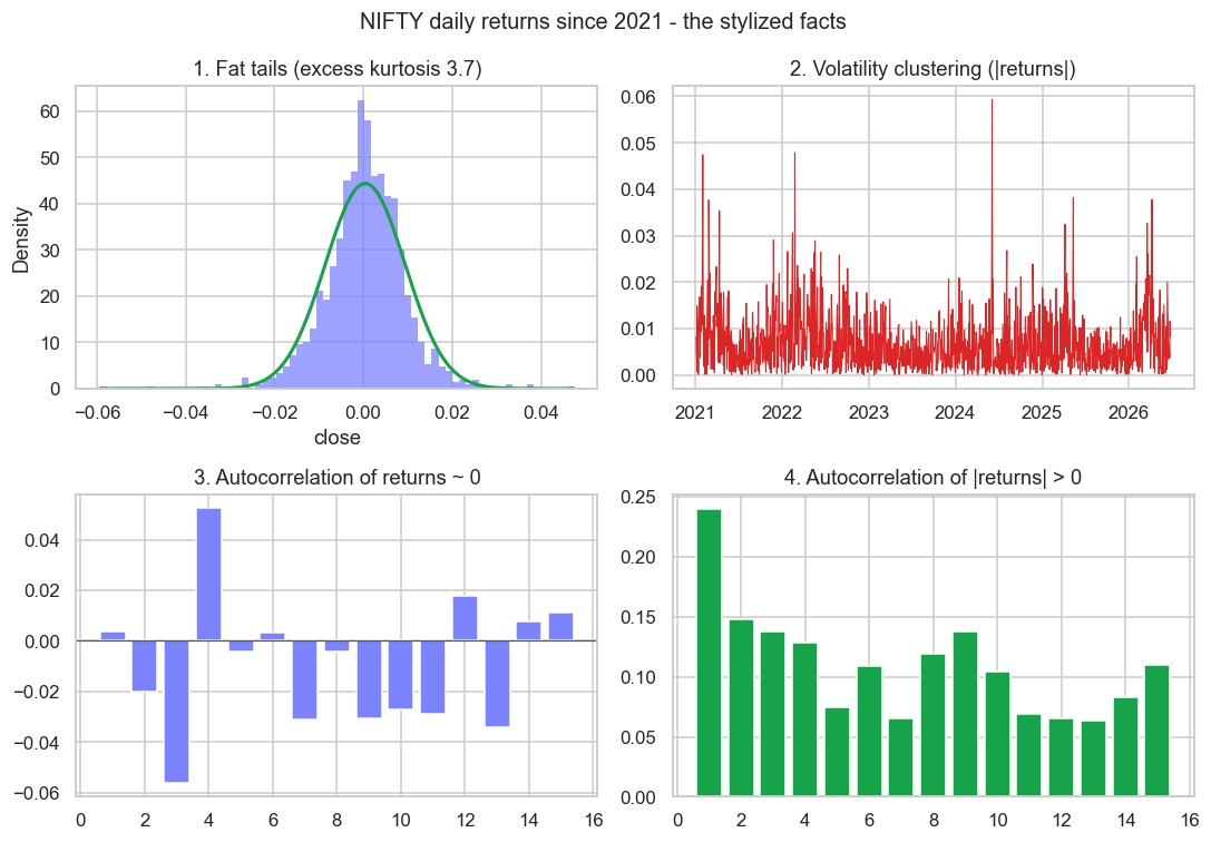
Read the four panels - each is a law of markets:

1. Fat tails. Real returns (purple) pile up taller in the middle and stretch far past the normal bell curve (green) at the edges. The excess kurtosis of ~3.7 confirms it: extreme days happen far more often than a "coin-flip" world allows.
2. Volatility clustering. The size of moves comes in runs - calm stretches and violent stretches, never evenly mixed. Big days cluster with big days.
3. Returns are nearly unpredictable. The autocorrelation of returns is essentially zero at every lag - yesterday's return tells you almost nothing about today's direction. This is the kernel of truth in the efficient-market idea.
4. But their size has memory. The autocorrelation of absolute returns is clearly positive and decays slowly - the magnitude of moves is highly predictable, even though the direction isn't.

Why this matters more than anything

Facts 3 and 4 together are the deepest insight in all of quantitative trading, so sit with them:

You cannot reliably predict the direction of returns. But you can predict their size - the volatility.

This asymmetry shapes everything that follows. It's why naive "predict tomorrow's return" strategies mostly fail (direction is near-random), and why the strategies that endure are built on what is predictable - volatility, risk, relationships between instruments. A huge slice of professional quant work isn't forecasting price at all; it's forecasting risk, because risk is the part of the market that actually has memory. We'll build exactly that model in Chapter 16.

The leverage effect

One more pattern, with a human cause. Volatility tends to rise more after the market falls than after it rises by the same amount - fear moves faster than greed. This is the leverage effect, and it's why a crash feels so much more violent than a rally: the down move and the spike in volatility arrive together. Any honest risk model has to account for this asymmetry between up and down.

Try it yourself

• Run the stylized-facts figure on a single volatile stock (say ADANIENT on NSE). Are its tails even fatter than the index's? (Single stocks usually are.)
• Compare the excess kurtosis of daily returns versus weekly returns (resample the price). Do the tails get thinner as you zoom out in time?
• Check the leverage effect directly: is average volatility in the 5 days after a 2% down day higher than after a 2% up day?

Recap

• A return has two forms: simple (intuitive, for humans) and log (adds across time, for maths) - identical for small moves, divergent for large ones.
• Returns obey four universal stylized facts: fat tails, volatility clustering, near-zero autocorrelation of returns, and positive autocorrelation of |returns|.
• The crucial asymmetry: you can't predict direction but you can predict size (volatility) - which is why durable quant strategies target risk, not price forecasts.
• The leverage effect means volatility spikes more after falls than rises - fear is faster than greed, and risk models must be asymmetric.

We now know what returns look like. Next we give ourselves the tools to reason about that randomness - probability, expectation, and the Monte Carlo simulation that lets a quant answer questions no formula can.