Quant Researcher vs Quant Trader vs Quant Developer

"Quant" is not one job. The word covers three very different people who sit a few desks apart, speak partly different languages, and are each responsible for a different slice of the same trade. One of them finds an edge in the data. One of them turns that edge into software that can survive a live market. One of them puts real money behind it and answers for the result. On a small team a single person wears all three hats badly; on a serious desk they are three careers. Confusing them is the single most common reason a beautiful backtest never makes a rupee. So before we go anywhere near the mathematics, let us meet the people who use it.

Three roles, one trade

The pipeline of a systematic strategy maps almost perfectly onto three titles.

The quant researcher finds the edge. Their raw material is data and their output is a signal - a precise, testable rule that says when the odds are tilted. They live in statistics, hypothesis testing, time series and a healthy paranoia about fooling themselves. Their deliverable is not money; it is evidence - a notebook that says "this pattern is real, here is how strong, here is how it could be wrong."

The quant developer (or quant engineer) builds the machine. They take the researcher's signal and turn it into a production system: clean data pipelines, an order gateway like OpenAlgo, state management, latency budgets, logging, recovery after a crash. Their world is software engineering with a market accent. A signal that the researcher ran once on a tidy CSV must now run every day, on live data, without leaking look-ahead, without double-firing an order, and without falling over when the feed hiccups.

The quant trader runs the book. They own the live risk: position sizing, stops, capital allocation, when to turn the strategy off, how to execute without moving the price against themselves. They answer for the profit and loss. A trader who does not understand the model is dangerous, and a model that no trader will stand behind never goes live.

What the researcher actually hands over

Let us make this concrete. A researcher is handed a question: does a simple trend rule beat just holding the index? They pull eleven years of NIFTY, build a 20-day versus 100-day moving-average cross, and measure it honestly - signal known at today's close, return earned tomorrow, no peeking.

# The researcher's job: turn raw NIFTY prices into one tested signal and report its edge honestly.
import os
from datetime import datetime

from openalgo import api, ta

client = api(
    api_key=os.getenv("OPENALGO_API_KEY", "your_api_key_here"),
    host=os.getenv("OPENALGO_HOST", "http://127.0.0.1:5000"),
)

end = datetime.now().strftime("%Y-%m-%d")
df = client.history(symbol="NIFTY", exchange="NSE_INDEX", interval="D",
                    start_date="2015-01-01", end_date=end)

close = df["close"]
fast = ta.sma(close, 20)
slow = ta.sma(close, 100)

# Signal is known at today's close; the return it earns is tomorrow's. No look-ahead.
long_today = fast > slow
fwd = close.pct_change().shift(-1)
mask = fast.notna() & slow.notna() & fwd.notna()

fwd_m = fwd[mask]
long_rets = fwd_m[long_today[mask]]

hit, avg = (long_rets > 0).mean(), long_rets.mean()
base_hit, base_avg = (fwd_m > 0).mean(), fwd_m.mean()

print(f"NIFTY daily, {int(mask.sum())} test days {df.index[mask][0].date()} to {df.index[mask][-1].date()}")
print(f"Signal: 20/100 SMA cross, long when fast > slow ({len(long_rets)} days in market)")
print(f"  Next-day hit rate when long  : {hit:6.2%}   (baseline, all days {base_hit:.2%})")
print(f"  Avg next-day return when long: {avg:+.4%}   (baseline, all days {base_avg:+.4%})")
print(f"  Research edge: hit rate       {(hit - base_hit) * 100:+.2f} pp, "
      f"return {(avg - base_avg) * 1e4:+.1f} bps/day")

NIFTY daily, 2744 test days 2015-05-28 to 2026-06-24
Signal: 20/100 SMA cross, long when fast > slow (1834 days in market)
  Next-day hit rate when long  : 54.47%   (baseline, all days 53.94%)
  Avg next-day return when long: +0.0440%   (baseline, all days +0.0440%)
  Research edge: hit rate       +0.54 pp, return -0.0 bps/day

The printout is the research deliverable. Over 2744 trading days from May 2015 to June 2026, the rule sat long for 1834 of them. On those long days the next session closed up 54.47% of the time, against a baseline of 53.94% on all days - an edge of just +0.54 percentage points in hit rate. The average next-day return when long was +0.0440%, identical to the all-days baseline to four decimals. So the directional edge is a whisper, and the per-day return edge is essentially nil.

A good researcher reports exactly that, without flattering it. They do not write "profitable trend system." They write "the cross adds almost no per-day return; what it mostly does is decide when to be in the market." That distinction is the whole job. The researcher's deliverable is calibrated honesty about how big the edge is and how easily it could be noise - a topic we treat properly in the chapter on multiple testing and false discovery (ch13).

The handoff, and the loop back

The signal now leaves the notebook. The developer wraps it in a system that fetches data, computes the same rule on the latest bar, sizes a position and routes an order - using the identical signal code the researcher wrote, so the backtest and the live bot can never silently disagree (the research-to-production parity we build in ch74). The trader then decides how much capital the strategy gets, what the kill-switch loss is, and whether today is a day to trade it at all.

The dashed red arrow is the part beginners forget. This is not a relay race where research hands off and walks away. The fills, the slippage, the days the strategy was switched off - all of that flows back to the researcher, who refines the next version. The best desks run this loop tightly, and the worst ones let research and trading drift into separate kingdoms that blame each other.

Where the edge meets reality

Now the same signal, seen through the developer's and trader's eyes. They do not care about the hit rate in a vacuum; they care what happens to actual money after costs. So we trade the rule for real: long when fast is above slow, flat otherwise, charged a realistic round-trip cost, and compared against simply buying and holding NIFTY.

Copy

# The developer/trader's job: take the SAME signal and see if it survives real round-trip costs.
import os
from datetime import datetime
from pathlib import Path

import matplotlib

matplotlib.use("Agg")
import matplotlib.pyplot as plt
import seaborn as sns
from openalgo import api, ta

client = api(
    api_key=os.getenv("OPENALGO_API_KEY", "your_api_key_here"),
    host=os.getenv("OPENALGO_HOST", "http://127.0.0.1:5000"),
)

end = datetime.now().strftime("%Y-%m-%d")
df = client.history(symbol="NIFTY", exchange="NSE_INDEX", interval="D",
                    start_date="2015-01-01", end_date=end)

close = df["close"]
fast, slow = ta.sma(close, 20), ta.sma(close, 100)

# Position decided at close (1 = long, 0 = flat), held the next day.
pos = (fast > slow).astype(float).shift(1).fillna(0.0)
ret = close.pct_change().fillna(0.0)

one_way = 0.0005                       # 5 bps each side: brokerage + STT + slippage (10 bps round trip)
turn = pos.diff().abs().fillna(0.0)    # 1.0 on every entry or exit
cost = turn * one_way

gross = (1 + pos * ret).cumprod()
net = (1 + pos * ret - cost).cumprod()
hold = (1 + ret).cumprod()
trips = int(turn.sum() / 2)

sns.set_theme(style="whitegrid")
fig, ax = plt.subplots(figsize=(10, 5.5))
ax.plot(df.index, gross, color="#7c83ff", lw=1.8, label="Strategy gross")
ax.plot(df.index, net, color="#dc2626", lw=1.8, label=f"Strategy net of {one_way*2*1e4:.0f} bps round trip")
ax.plot(df.index, hold, color="#9a9a9a", lw=1.2, ls="--", label="Buy & hold NIFTY")
ax.set_title("Same signal, two jobs: research vs the cost of trading it (NIFTY 20/100 SMA)")
ax.set_ylabel("Growth of 1 rupee")
ax.legend(loc="upper left")
fig.tight_layout()
out = Path(__file__).with_suffix(".png")
plt.savefig(out, dpi=110, bbox_inches="tight")

print(f"{trips} round-trip trades over {len(close)} days. "
      f"Final wealth -> gross {gross.iloc[-1]:.2f}x, net {net.iloc[-1]:.2f}x, buy&hold {hold.iloc[-1]:.2f}x. "
      f"Costs ate {(gross.iloc[-1] - net.iloc[-1]):.2f}x. Saved {out.name}")

Live output

14 round-trip trades over 2844 days. Final wealth -> gross 2.10x, net 2.07x, buy&hold 2.90x. Costs ate 0.03x. Saved 02_costs_equity.png

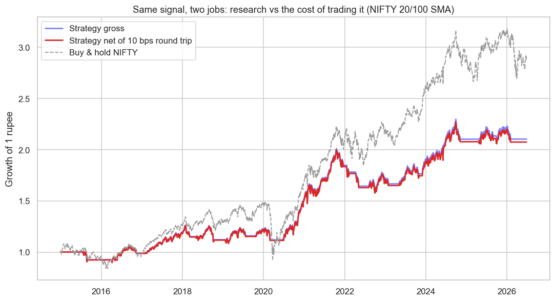
The result is sobering and completely honest. The signal made one rupee grow to 2.10x gross. After a 10 basis-point round-trip cost (brokerage plus transaction tax plus a little slippage, charged 5 bps each side) it made 2.07x net. Costs alone ate only 0.03x - almost nothing - because this slow rule traded just 14 round trips in eleven years. Low turnover is cheap. So far the developer's verdict is "it survives costs."

Then the trader looks at the grey dashed line and winces: buy and hold made 2.90x. The strategy that looked like it had an edge in research underperformed the laziest possible benchmark. What it really bought was not return but drawdown avoidance - notice the equity curve going flat through the 2020 crash and the 2022 fall, exactly when it was sitting out. Whether that is worth giving up a third of your wealth is a trader's judgement, not a researcher's.

Notice also the hidden lesson about turnover. This signal survived costs only because it trades 14 times. Replace the 100-day average with a 5-day one and the same code would flip hundreds of times, and at 10 bps a flip the costs alone would bury it long before any benchmark argument. The developer who knows this, and the trader who feels it in the P&L, are worth as much as the researcher who found the pattern.

Execution quants, alpha quants, and where you fit

Two more labels you will hear. An alpha quant is a researcher specialised in finding signals - the predictive edge itself. An execution quant sits between developer and trader, specialised in getting filled cheaply: minimising market impact, slicing large orders, beating a benchmark price like VWAP. On a high-frequency desk these split further into hardware, networking and microstructure specialists, because at microsecond scale execution is the alpha. On a small systematic shop, one person may research, code and trade all three - which is exactly the path an OpenAlgo-based retail quant walks.

If you are deciding which to become: the researcher path rewards statistics and scepticism, the developer path rewards clean systems thinking, the trader path rewards risk temperament and a strong stomach. Most durable careers start by being genuinely good at one and literate in the other two - because, as the next chapters on firm types (ch03) and participants (ch05) will show, the whole industry is organised around this division of labour. Learn to respect all three, and you will stop writing backtests that die the moment real money touches them.