Market Participants and Who Moves Prices

Every tick on your screen is the residue of an argument. Somebody wanted to buy badly enough to lift the offer, or sell badly enough to hit the bid, and the print is who won. So before we model prices, we should ask the blunt question that beginners skip and professionals never stop asking: who is on the other side of my trade, and what do they know that I do not? The market is not a weather system that just happens to you. It is a crowd of very different participants, each with different goals, horizons and information. Learn to tell them apart and the tape starts to make sense.

The cast of characters

A handful of participant types account for almost all Indian market activity, and each leaves a different signature.

• Retail traders - individuals trading their own money. Huge in count, small per ticket, and concentrated in options and intraday equity. As a group, retail flow is mostly uninformed: it reacts to price rather than anticipating it, and it is the liquidity that faster players feed on.
• HNIs and the proprietary desks that resemble them - high net worth individuals and firm capital trading for short-term edge. More sophisticated, more leveraged, often the bridge between retail noise and institutional signal.
• FPIs - foreign portfolio investors. Large, trend-setting, and the single most watched flow in Indian equities. When FPIs turn net buyers or sellers for weeks, the index usually follows.
• DIIs - domestic institutional investors: mutual funds, insurers, pension money. Often the counterweight to FPIs, absorbing foreign selling with steady domestic inflows. The FPI-versus-DII tug of war is the macro story of most Indian quarters.
• Market makers - participants who quote both a bid and an ask continuously, earning the spread for supplying liquidity. They rarely want a directional view; they want flow and a flat book by the close. We devote much of Module C and chapter 38 to their world.

Informed versus uninformed flow

The deepest cut through the crowd is not retail-versus-institution but informed versus uninformed. Informed flow trades ahead of information - it buys because it expects the price to rise, and its trades predict the next move. Uninformed flow trades for reasons unrelated to future price: rebalancing, hedging, liquidity needs, or simply chasing what already happened.

This distinction is the engine of microstructure. A market maker's nightmare is adverse selection - getting filled by someone who knows more, so that every trade you win is one you wish you had lost. Makers protect themselves by widening spreads when flow looks toxic and tightening them when it looks benign. As a quant, your entire problem is to be on the informed side often enough, after costs, to matter. Most retail strategies quietly sit on the uninformed side and pay for the privilege.

The price of fear

Here is the honest problem: India does not hand you clean, real-time, participant-tagged order flow. Exchanges publish a daily FPI-versus-DII cash figure and the F&O client-category turnover, but nothing tick-by-tick that says "a fund just bought." So a working quant reaches for proxies - observable series that move with the participants you cannot see directly. The best-known proxy for crowd fear is India VIX, the index of expected 30-day volatility implied by the NIFTY option chain. When the crowd reaches for protection, option prices swell and VIX rises. So VIX is, quite literally, the price of fear.

# The crowd's fear, measured: how NIFTY returns move against India VIX.
import os
from datetime import datetime, timedelta

import numpy as np
import pandas as pd
from openalgo import api

client = api(
    api_key=os.getenv("OPENALGO_API_KEY", "your_api_key_here"),
    host=os.getenv("OPENALGO_HOST", "http://127.0.0.1:5000"),
)

end = datetime.now().strftime("%Y-%m-%d")
start = (datetime.now() - timedelta(days=365)).strftime("%Y-%m-%d")

nifty = client.history(symbol="NIFTY", exchange="NSE_INDEX", interval="D",
                       start_date=start, end_date=end)["close"]
vix = client.history(symbol="INDIAVIX", exchange="NSE_INDEX", interval="D",
                     start_date=start, end_date=end)["close"]

# Align: NIFTY daily return vs same-day change in India VIX (the "price of fear").
df = pd.concat([nifty.pct_change(), vix.pct_change(), vix.diff()], axis=1).dropna()
df.columns = ["nifty_ret", "vix_pct", "vix_pts"]

corr = df["nifty_ret"].corr(df["vix_pct"])
slope = np.polyfit(df["nifty_ret"], df["vix_pts"], 1)[0]  # VIX points per 1.0 of NIFTY return

down = df[df["nifty_ret"] < 0]["vix_pts"].mean()   # avg VIX move on red days
up = df[df["nifty_ret"] > 0]["vix_pts"].mean()     # avg VIX move on green days

print(f"Window: {len(df)} trading days, {df.index[0].date()} to {df.index[-1].date()}")
print(f"India VIX latest close   : {vix.iloc[-1]:.2f}  (annualised expected move)")
print(f"Corr(NIFTY ret, VIX chg) : {corr:+.3f}   <- the inverse 'price of fear'")
print(f"Sensitivity              : a -1% NIFTY day lifts VIX by ~{-slope/100:.3f} pts")
print(f"Avg VIX change, red days : {down:+.3f} pts")
print(f"Avg VIX change, green days: {up:+.3f} pts   <- fear rises faster than it falls")

Window: 244 trading days, 2025-07-01 to 2026-06-25
India VIX latest close   : 13.05  (annualised expected move)
Corr(NIFTY ret, VIX chg) : -0.731   <- the inverse 'price of fear'
Sensitivity              : a -1% NIFTY day lifts VIX by ~0.899 pts
Avg VIX change, red days : +0.443 pts
Avg VIX change, green days: -0.413 pts   <- fear rises faster than it falls

Over the last 244 trading days the correlation between NIFTY's daily return and the change in India VIX came out at -0.731 - strongly negative, exactly as the story predicts. Down days are fear days. The regression puts a number on it: a one-percent fall in NIFTY lifts VIX by roughly 0.9 points on average. And notice the asymmetry the script prints - VIX rose about +0.44 points on red days but fell only -0.41 on green days of similar size. Fear arrives faster than calm returns. That is the leverage effect of chapter 9 showing up in participant behaviour: protection is bid for in a panic and sold back only grudgingly. With VIX sitting near 13 as this ran, the crowd was pricing a calm month - which, as every options seller learns, is precisely when complacency is cheapest and most dangerous.

Footprints in volume

If you cannot see participants directly, you can often see where they stepped. Large institutions cannot accumulate a position quietly forever; sooner or later their buying or selling shows up as a volume spike far above the stock's normal turnover. Volume is the most democratic footprint on the tape - it is reported in full, for every name, every day.

Copy

# Footprints in volume: marking the days large participants showed up in RELIANCE.
import os
from datetime import datetime, timedelta
from pathlib import Path

import matplotlib

matplotlib.use("Agg")
import matplotlib.pyplot as plt
import seaborn as sns
from openalgo import api

client = api(
    api_key=os.getenv("OPENALGO_API_KEY", "your_api_key_here"),
    host=os.getenv("OPENALGO_HOST", "http://127.0.0.1:5000"),
)

end = datetime.now().strftime("%Y-%m-%d")
start = (datetime.now() - timedelta(days=365)).strftime("%Y-%m-%d")
df = client.history(symbol="RELIANCE", exchange="NSE", interval="D",
                    start_date=start, end_date=end)

vol = df["volume"]
close = df["close"]
med = vol.rolling(20, min_periods=10).median()      # a participant-neutral baseline
spike = vol > 2 * med                                # days big money likely stepped in

sns.set_theme(style="whitegrid")
fig, (axp, axv) = plt.subplots(2, 1, figsize=(10, 7), sharex=True,
                               gridspec_kw={"height_ratios": [2, 1]})

axp.plot(df.index, close, color="#7c83ff", lw=1.4)
axp.scatter(df.index[spike], close[spike], color="#dc2626", s=40, zorder=5, label="volume spike")
axp.set_title("RELIANCE daily close - red dots mark unusually high-volume days")
axp.set_ylabel("Close (Rs)")
axp.legend(loc="upper left")

axv.bar(df.index, vol / 1e6, color="#9aa0b5", width=1.0)
axv.bar(df.index[spike], vol[spike] / 1e6, color="#dc2626", width=1.0)
axv.plot(df.index, med / 1e6, color="#16a34a", lw=1.2, label="20-day median volume")
axv.set_ylabel("Volume (mn)")
axv.legend(loc="upper left")

fig.suptitle("Who moved the price? High-volume days as participant footprints", fontsize=13)
fig.tight_layout()
out = Path(__file__).with_suffix(".png")
plt.savefig(out, dpi=110, bbox_inches="tight")

big = vol.nlargest(1)
print(f"{len(df)} days, {int(spike.sum())} volume-spike days (>2x 20d median). "
      f"Biggest: {big.index[0].date()} at {int(big.iloc[0]/1e6)}mn shares on a "
      f"{close.pct_change().loc[big.index[0]]*100:+.2f}% day. Saved {out.name}")

Live output

245 days, 12 volume-spike days (>2x 20d median). Biggest: 2026-05-29 at 42mn shares on a -2.17% day. Saved 02_volume_footprints.png

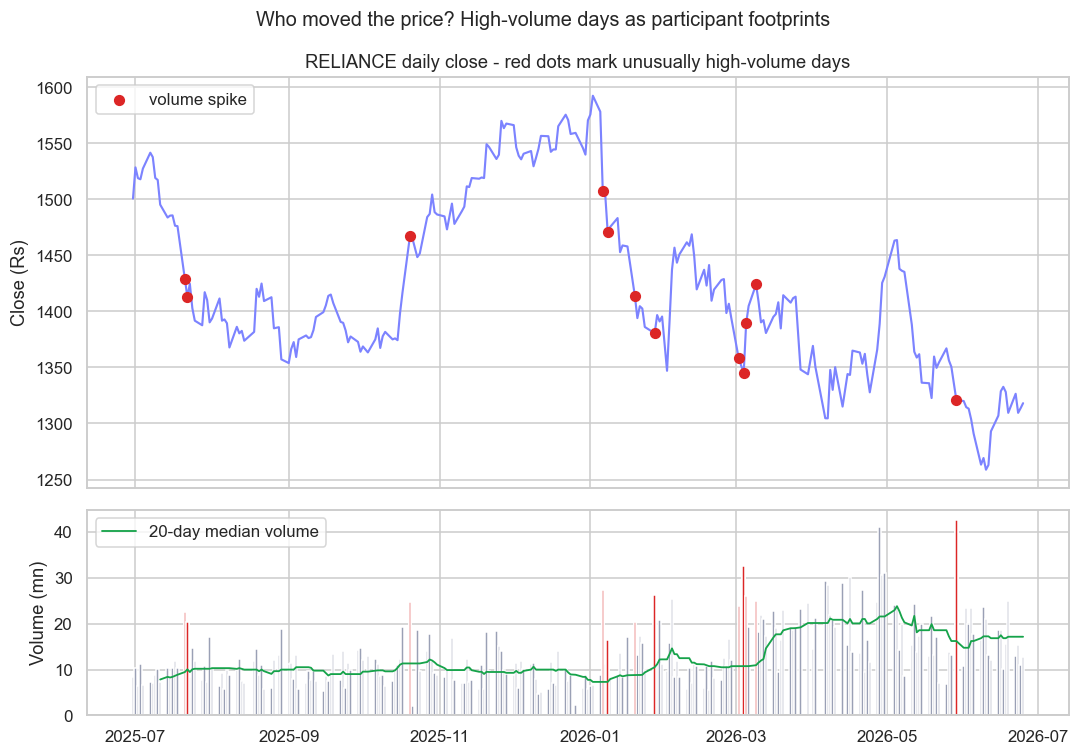
Across a year of RELIANCE, 12 of 245 days printed more than twice the 20-day median volume. The single biggest was 29 May 2026 at 42 million shares on a -2.17% day - the classic signature of large sellers hitting the market, the kind of distribution that retail rarely produces on its own. Mark those red dots against price and a pattern emerges: spikes cluster around results, index rebalancing and the bulk and block deals we study in chapter 24. They do not tell you who traded - volume is symmetric, every buyer has a seller - but they reliably flag that a big participant was active, which days deserve a second look, and which quiet days are just the crowd talking to itself.

What you can and cannot actually see

It is worth being blunt about the limits, because pretending otherwise is how quants fool themselves. You can see end-of-day FPI and DII cash flows, F&O client-category turnover, open interest, delivery percentages, bulk and block deals, and of course price and volume. You cannot see, in real time, who is buying, their intent, or their full size - much of it is sliced into child orders or routed through the derivatives book precisely to stay invisible. So every participant signal you build is an inference from a proxy, with a confidence attached, not a fact.

That mindset - triangulating hidden flow from observable proxies, always with honest uncertainty - is the heart of flow-based trading, which we develop fully in chapter 64. For now, carry one idea forward: the price you see is the outcome of a contest between providers and takers, informed and uninformed, foreign and domestic. Next, in chapter 6, we follow a single order from your screen all the way to the exchange matching engine, and watch exactly how that contest is settled, one fill at a time.