The Research-to-Production Pipeline

A backtest is a promise: run this logic on the past and it would have made money. Live trading is the moment that promise is tested with real capital. Between the two sits a gap where most strategies quietly break - not because the idea was wrong, but because the code that traded live was never quite the code that was tested. A parameter drifted. A rolling window was computed differently. The research notebook used the full series; the live bot saw only the last bar and rounded a corner. This chapter is about closing that gap by design, so that the thing you tested and the thing you trade are provably the same thing.

The research-production gap

In a research notebook you have the luxury of the whole dataset at once. You load years of NIFTY bars, vectorise an indicator across the entire array, and read off a Sharpe ratio. It is fast, exploratory, and forgiving. Live trading is the opposite world: bars arrive one at a time, you hold only a trailing window in memory, latency matters, and a crash at 9:20 is a real loss, not a re-run.

The research-production gap is the set of subtle differences between these two worlds that cause a live strategy to behave unlike its backtest. The classic culprits: a signal reimplemented in a "production language" by a different person; an indicator whose warm-up period is handled one way in research and another live; a parameter hard-coded in the notebook but typed by hand into the live config; a timestamp that is bar-close in the backtest but bar-open live. Each is small. Together they mean your live P&L is sampling a different strategy than the one you validated.

One signal, two callers

The fix is structural, not heroic: write the signal logic once, in a shared module, and have both the backtest and the live process import the same function. No copy-paste, no reimplementation, no "production version". The research harness calls signal(df) on all of history; the live loop calls the identical signal(df) on its trailing window and takes the last value. Same function, same parameters, two callers.

The example below makes this concrete. A single signal(df) function - a 20/50 SMA cross returning +1 long or -1 short - is defined once and run twice: across the full NIFTY history (the backtest) and on just the trailing window a live process would hold (the live decision).

# One signal, two contexts: the SAME signal(df) runs the backtest and the live decision.
import os
from datetime import datetime

import numpy as np
import pandas as pd
from openalgo import api, ta

client = api(
    api_key=os.getenv("OPENALGO_API_KEY", "your_api_key_here"),
    host=os.getenv("OPENALGO_HOST", "http://127.0.0.1:5000"),
)

# --- CONFIG: parameters live in one place, shared by backtest and live ---
CONFIG = {"fast": 20, "slow": 50, "live_window": 250}


def signal(df, fast=CONFIG["fast"], slow=CONFIG["slow"]):
    """Vectorised position: +1 long when fast SMA > slow SMA, else -1 short.
    This is the ONLY copy of the logic. Backtest and live both call it."""
    close = df["close"]
    pos = pd.Series(np.where(ta.sma(close, fast) > ta.sma(close, slow), 1, -1),
                    index=df.index)
    return pos


end = datetime.now().strftime("%Y-%m-%d")
df = client.history(symbol="NIFTY", exchange="NSE_INDEX", interval="D",
                    start_date="2023-01-01", end_date=end)

# --- BACKTEST: apply the signal across the full history ---
bt = signal(df)
trades = int((bt.diff() != 0).sum()) - 1                 # number of position flips
bt_decision = int(bt.iloc[-1])

# --- LIVE: the bot holds only a trailing window in memory, not all of history ---
window = df.tail(CONFIG["live_window"])                   # what a live process keeps
live_decision = int(signal(window).iloc[-1])             # decide on the latest bar

# --- PARITY: identical code path must give an identical answer ---
overlap = bt.tail(120)                                   # compare the shared tail
agree_tail = bool((signal(df.tail(CONFIG["live_window"])).tail(120).values
                   == overlap.values).all())

label = {1: "LONG", -1: "SHORT"}
print(f"NIFTY daily {df.index[0].date()} -> {df.index[-1].date()}  ({len(df)} bars)")
print(f"Signal: {CONFIG['fast']}/{CONFIG['slow']} SMA cross  (one signal() function)")
print(f"  Backtest position changes : {trades}")
print(f"  Backtest last bar decision: {label[bt_decision]}  @ {df['close'].iloc[-1]:.2f}")
print(f"  Live  (trailing {CONFIG['live_window']}) decision: {label[live_decision]}")
print(f"  Decisions match           : {bt_decision == live_decision}")
print(f"  Last 120 bars match too   : {agree_tail}")
print("\nSame code, same data, same answer - backtest-live parity by construction.")

NIFTY daily 2023-01-02 -> 2026-06-25  (862 bars)
Signal: 20/50 SMA cross  (one signal() function)
  Backtest position changes : 14
  Backtest last bar decision: SHORT  @ 24056.00
  Live  (trailing 250) decision: SHORT
  Decisions match           : True
  Last 120 bars match too   : True

Same code, same data, same answer - backtest-live parity by construction.

Over 862 NIFTY daily bars from 2 January 2023, the signal flips position 14 times. Its last-bar backtest decision is SHORT at 24056.00 - and the live process, computing from only its trailing 250-bar window, also returns SHORT. The two decisions match, and so do the last 120 bars where the windows overlap. That agreement is not luck; it is what you get for free when there is only one copy of the logic.

Config, parameters and parity

Notice where the parameters live in that example: in a single CONFIG dict, read by the one signal function. This is the second discipline. Configuration - the fast and slow lengths, thresholds, instrument, position cap - belongs in one place that both backtest and live read, never hard-coded in two. If research sweeps slow = 50 and live runs slow = 55 because someone fat-fingered the live config, you are trading an untested strategy and your backtest is a fiction.

Backtest-live parity is the property that the live system, fed the same inputs, produces the same outputs as the backtest. It is worth testing explicitly and continuously: every day, recompute the live signal path on yesterday's bars and assert it equals what the backtest produces on the same window. When they diverge, something has drifted - a data revision, a library upgrade, a timezone change - and you want to find out from a failing parity check, not from a mysterious live loss.

Parity also disciplines how you treat time. The most common silent break is the look-ahead seam (Chapter 68): in research it is tempting to compute a signal on a bar's close and, sloppily, act on that same bar. Live, that bar's close does not exist until the bar is over. If the shared function only ever uses information available at decision time - prior closes, the current bar's open - then backtest and live cannot disagree about what was knowable when.

Staging, deployment and the path to live

You do not move from notebook to real money in one jump. A sane pipeline has stages, each a higher bar of trust:

• Research - free exploration on historical data, the place ideas are born and most die.
• Backtest - the shared signal run over a clean, point-in-time history (Chapter 73), with honest costs.
• Sandbox - the same code wired to live data but to a simulated broker. In OpenAlgo this is analyzer mode: orders are generated and tracked but never reach a real exchange. This catches the bugs a backtest cannot - bad ticks, API timeouts, rate limits, malformed orders - with zero financial risk.
• Paper-to-small - live with real orders but tiny size, to measure real slippage and fills against the backtest's assumptions.
• Full size - only after the live track record matches the backtest within tolerance.

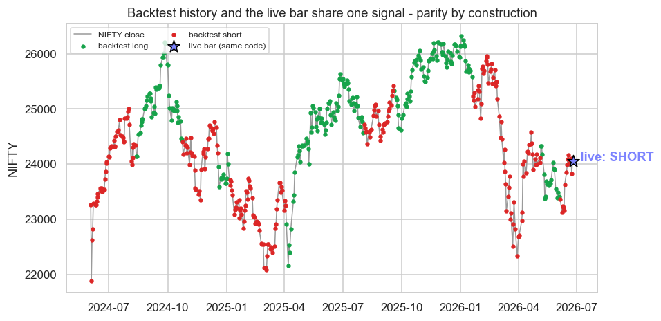
A strategy earns promotion to the next stage by evidence, not enthusiasm. The chart below shows the same shared signal on NIFTY history with the latest live bar appended in a distinct colour - the live point is not a new computation, it is the same signal() evaluated on the newest bar, sitting on the very curve the backtest drew.

Copy

# Parity, drawn: the backtest signal over history, with the latest live point appended in a distinct colour.
import os
from datetime import datetime
from pathlib import Path

import matplotlib

matplotlib.use("Agg")
import matplotlib.pyplot as plt
import numpy as np
import pandas as pd
import seaborn as sns
from openalgo import api, ta

client = api(
    api_key=os.getenv("OPENALGO_API_KEY", "your_api_key_here"),
    host=os.getenv("OPENALGO_HOST", "http://127.0.0.1:5000"),
)

CONFIG = {"fast": 20, "slow": 50}


def signal(df):
    """The shared signal: +1 long when fast SMA > slow SMA, else -1 short."""
    close = df["close"]
    return pd.Series(np.where(ta.sma(close, CONFIG["fast"]) > ta.sma(close, CONFIG["slow"]),
                              1, -1), index=df.index)


end = datetime.now().strftime("%Y-%m-%d")
df = client.history(symbol="NIFTY", exchange="NSE_INDEX", interval="D",
                    start_date="2024-06-01", end_date=end)

pos = signal(df)
hist, live = df.iloc[:-1], df.iloc[-1:]                   # all-but-last vs the live bar
live_pos = int(signal(df).iloc[-1])                      # live decision from same code

sns.set_theme(style="whitegrid")
fig, ax = plt.subplots(figsize=(9, 4.6))
ax.plot(hist.index, hist["close"], color="#9a9a9a", lw=1.0, zorder=1, label="NIFTY close")

# Colour the backtest by the signal's position state - this is what research saw
long_m = pos.iloc[:-1] == 1
ax.scatter(hist.index[long_m], hist["close"][long_m], s=10, color="#16a34a", label="backtest long")
ax.scatter(hist.index[~long_m], hist["close"][~long_m], s=10, color="#dc2626", label="backtest short")

# The latest LIVE point, same signal, drawn in a distinct colour on the same curve
ax.scatter(live.index, live["close"], s=140, color="#7c83ff", edgecolor="black",
           zorder=5, marker="*", label="live bar (same code)")
ax.annotate(f"  live: {'LONG' if live_pos == 1 else 'SHORT'}",
            (live.index[-1], live["close"].iloc[-1]), color="#7c83ff", fontweight="bold")

ax.set_title("Backtest history and the live bar share one signal - parity by construction")
ax.set_ylabel("NIFTY")
ax.legend(loc="upper left", fontsize=8, ncol=2)
out = Path(__file__).with_suffix(".png")
plt.savefig(out, dpi=110, bbox_inches="tight")
print(f"NIFTY {df.index[0].date()} -> {df.index[-1].date()}: live bar decision "
      f"{'LONG' if live_pos == 1 else 'SHORT'}, same signal() as the backtest. Saved {out.name}")

Live output

NIFTY 2024-06-03 -> 2026-06-25: live bar decision SHORT, same signal() as the backtest. Saved 02_parity_chart.png

Versioning and rollback

Finally, the unglamorous safety net. Every component must be versioned: the code (a git commit), the parameters (the config file), and the data window (Chapter 73's point-in-time store). A live trade should be traceable to the exact code commit and config that produced it. Then, when a deploy goes wrong - a refactor that breaks parity, a parameter change that bleeds money - you can roll back to the last known-good version instantly, the way any production engineer would.

With a strategy that crosses the research-production divide intact, the next question is the machinery around it - the order and position management, the event loop, and recovery after a crash. That live trading system is Chapter 75.