Walk-Forward, Purged CV and Deflated Sharpe

A single train/test split answers exactly one question: did this strategy work on this one particular slice of the future. But you do not trade one future. You trade a rolling sequence of them - fit on what you know, deploy, watch it age, re-fit, deploy again. A validation scheme that respects the clock has to imitate that loop, and most do not. The previous chapters taught you to lag your signals and audit your data; this one is about the harder discipline of testing in time, where the very tools that work beautifully on independent data - shuffling, k-fold cross-validation - quietly leak the future into the past and hand you a Sharpe that evaporates the day you go live.

Walk-forward: validation that respects the clock

The honest baseline is walk-forward analysis. You fit the strategy (choose its parameters, train its model) on a stretch of history, then judge it on the next unseen slice, then slide the window forward and repeat. The training window can be expanding (always start from the beginning, so it grows) or rolling (fixed length, so it forgets the distant past). Either way the rule is sacred: the strategy is never scored on a bar it could have seen while fitting.

Let us run a real one. We let a simple momentum rule - long when price is above its SMA, short below - choose its own lookback from a grid of 10 to 200 days, fitting on everything seen so far by maximising in-sample Sharpe, then grade it only on the next unseen block, six times over.

# Walk-forward: pick the SMA lookback in-sample, score it out-of-sample, fold after fold.
import os
from datetime import datetime

import numpy as np
import pandas as pd
from openalgo import api

client = api(
    api_key=os.getenv("OPENALGO_API_KEY", "your_api_key_here"),
    host=os.getenv("OPENALGO_HOST", "http://127.0.0.1:5000"),
)

end = datetime.now().strftime("%Y-%m-%d")
c = client.history(symbol="NIFTY", exchange="NSE_INDEX", interval="D",
                   start_date="2015-01-01", end_date=end)["close"]
r = c.pct_change()
ann = np.sqrt(252.0)

grid = [10, 20, 50, 100, 150, 200]          # candidate SMA lookbacks to fit
# Pre-compute the lagged P&L of every candidate once (signal known strictly before the bar).
pnl = {L: (np.sign(c - c.rolling(L).mean()).shift(1) * r) for L in grid}


def sharpe(x):
    x = x.dropna()
    return x.mean() / x.std() * ann if len(x) > 5 else np.nan


n, folds = len(c), 6
edges = np.linspace(int(n * 0.4), n, folds + 1, dtype=int)   # expanding train, 6 OOS blocks
oos_all, rows = [], []
for k in range(folds):
    tr_end, te_end = edges[k], edges[k + 1]
    best = max(grid, key=lambda L: sharpe(pnl[L].iloc[:tr_end]))   # fit on the past only
    oos = pnl[best].iloc[tr_end:te_end]                            # score on the unseen block
    oos_all.append(oos)
    rows.append((k + 1, c.index[tr_end].date(), c.index[te_end - 1].date(), best, sharpe(oos)))

agg = sharpe(pd.concat(oos_all))
print(f"Walk-forward on NIFTY daily, {n} bars, expanding train -> 6 out-of-sample folds")
print(f"{'fold':>4} {'OOS start':>12} {'OOS end':>12} {'fitted SMA':>11} {'OOS Sharpe':>11}")
for f, s, e, L, sh in rows:
    print(f"{f:>4} {str(s):>12} {str(e):>12} {L:>11} {sh:>+11.2f}")
mean_fold = np.nanmean([row[4] for row in rows])
print(f"\nMean per-fold OOS Sharpe {mean_fold:+.2f}; aggregate stitched-OOS Sharpe {agg:+.2f}.")

Walk-forward on NIFTY daily, 2844 bars, expanding train -> 6 out-of-sample folds
fold    OOS start      OOS end  fitted SMA  OOS Sharpe
   1   2019-08-06   2020-09-28          10       -0.07
   2   2020-09-29   2021-11-23          50       +0.70
   3   2021-11-24   2023-01-11         100       -0.77
   4   2023-01-12   2024-03-05          50       +1.64
   5   2024-03-06   2025-05-02          50       +0.25
   6   2025-05-05   2026-06-25          50       -0.71

Mean per-fold OOS Sharpe +0.17; aggregate stitched-OOS Sharpe +0.06.

The result is a lesson in humility. Across 2844 NIFTY bars the in-sample fit almost always preferred an SMA of 50, yet out of sample that same rule swung from -0.77 to +1.64 fold by fold: -0.07, +0.70, -0.77, +1.64, +0.25, -0.71. One spectacular stretch through 2023 to 2024 is flanked on both sides by losers. The mean per-fold Sharpe is a feeble +0.17 and the aggregate, stitching all six out-of-sample blocks into one P&L stream, is +0.06 - a coin flip. A single lucky split could have shown you only the +1.64 and you would have funded it. Walk-forward shows you the whole distribution of futures, and its verdict here is blunt: no durable edge.

Why ordinary k-fold cross-validation leaks

Machine-learning practitioners reach instinctively for k-fold cross-validation: shuffle the rows, cut them into k folds, train on k-1 and test on the one held out, rotate, average. On independent observations it is the gold standard. On a price series it is a disaster, for two reasons.

First, shuffling destroys the arrow of time. After a shuffle, the training set contains bars from after the test bars, so the model is quite literally fitted on the future to predict the past. That is look-ahead bias dressed up as best practice. Second, and more subtly, even contiguous folds leak at their seams. Quant labels are rarely about a single bar. If you label a day by its forward five-day return, the label attached to the last training bar overlaps the first few test bars. Features built from trailing windows do the same on the other side. Serial correlation means neighbouring observations are near-duplicates, so a test fold sitting flush against a train fold has effectively already been seen. The cross-validation score comes back glowing, and it is a mirage.

Purged k-fold and the embargo

The fix, due to Lopez de Prado, is purged k-fold cross-validation. Keep the folds in time order, but before training, purge from the training set any observation whose label window overlaps the test interval. That removes the seam leakage at a stroke. Then add an embargo: drop a further band of training observations immediately after each test block, because serial correlation means the bars just after the test still carry information that bled out of it. Purge handles the label overlap; the embargo handles the autocorrelation that purge alone misses.

Drawn over a real timeline, the geometry is easy to see: the test block slides forward fold by fold, the purge bands hug it on both sides, and the embargo trails just behind.

Copy

# Purged k-fold CV over a real NIFTY timeline: train, purge, embargo and test blocks.
import os
from datetime import datetime
from pathlib import Path

import matplotlib

matplotlib.use("Agg")
import matplotlib.patches as mpatches
import matplotlib.pyplot as plt
import seaborn as sns
from openalgo import api

client = api(
    api_key=os.getenv("OPENALGO_API_KEY", "your_api_key_here"),
    host=os.getenv("OPENALGO_HOST", "http://127.0.0.1:5000"),
)

end = datetime.now().strftime("%Y-%m-%d")
idx = client.history(symbol="NIFTY", exchange="NSE_INDEX", interval="D",
                     start_date="2018-01-01", end_date=end).index
n = len(idx)                       # real number of trading bars on the time axis
k = 5                              # folds
purge = max(3, n // 60)            # bars dropped each side of test (label overlap)
embargo = max(2, n // 90)          # extra bars frozen right after the test block
size = n // k

cols = {"train": "#16a34a", "purge": "#e0852b", "embargo": "#9a9a9a", "test": "#7c83ff"}
sns.set_theme(style="whitegrid")
fig, ax = plt.subplots(figsize=(8.5, 4.6))

for f in range(k):
    y, ts, te = f, f * size, (f + 1) * size if f < k - 1 else n
    spans = {c: [] for c in cols}
    pl, pr = max(0, ts - purge), min(n, te + purge)        # purge bands hug the test block
    emb = min(n, pr + embargo)                              # embargo follows the right purge
    spans["test"].append((ts, te - ts))
    if ts > pl: spans["purge"].append((pl, ts - pl))
    if pr > te: spans["purge"].append((te, pr - te))
    if emb > pr: spans["embargo"].append((pr, emb - pr))
    if pl > 0: spans["train"].append((0, pl))              # remaining history is train
    if n > emb: spans["train"].append((emb, n - emb))
    for c in ("train", "purge", "embargo", "test"):
        ax.broken_barh(spans[c], (y - 0.4, 0.8), facecolors=cols[c], edgecolor="white", lw=0.4)

ax.set_yticks(range(k)); ax.set_yticklabels([f"fold {i + 1}" for i in range(k)])
ax.set_xlabel(f"trading bar index ({idx[0].date()} to {idx[-1].date()})")
ax.set_title("Purged k-fold cross-validation: test slides, purge and embargo seal the leak")
ax.invert_yaxis()
ax.legend(handles=[mpatches.Patch(color=v, label=lab) for lab, v in
                   [("train", cols["train"]), ("purge", cols["purge"]),
                    ("embargo", cols["embargo"]), ("test", cols["test"])]],
          loc="upper center", bbox_to_anchor=(0.5, -0.16), ncol=4, frameon=False)

out = Path(__file__).with_suffix(".png")
plt.savefig(out, dpi=110, bbox_inches="tight")
print(f"Purged {k}-fold over {n} NIFTY bars: test {size}, purge {purge}/side, embargo {embargo}. Saved {out.name}")

Live output

Purged 5-fold over 2101 NIFTY bars: test 420, purge 35/side, embargo 23. Saved 02_purged_cv_diagram.png

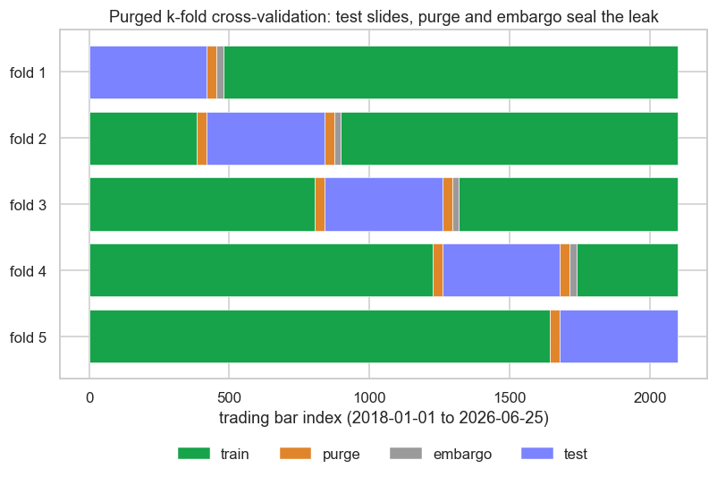
Here 2101 NIFTY bars are cut into five folds of 420, with 35 bars purged on each side of every test block and a 23-bar embargo following it. Those gaps look small, but they are the difference between a model that has genuinely never seen the test data and one that has been quietly fed its answers through the seam.

Combinatorial purged CV

Walk-forward and purged k-fold still give you a single backtest path through history, and a single path is a single sample - high variance, easy to over-read. Combinatorial purged cross-validation (CPCV) generalises the idea. Instead of holding out one test group at a time, you split the data into N groups and hold out every combination of k of them, purging and embargoing each. The N-choose-k combinations recombine into many distinct backtest paths rather than one, so you get a whole distribution of out-of-sample performance from the same data. From that distribution you can estimate the probability of backtest overfitting - the chance that the configuration which looked best in-sample is actually below median out-of-sample. A point estimate cannot tell you that; a distribution can.

Deflating the Sharpe for the search

Even a leak-free out-of-sample Sharpe still needs the haircut we built in Chapter 13. Every lookback on your grid, every fold split, every embargo length you tried is a trial, and the best of many trials is inflated by selection alone. The deflated Sharpe ratio of Bailey and Lopez de Prado turns that intuition into a probability: it takes your observed Sharpe, the number of independent trials, the variance of Sharpes across those trials, and the skew and kurtosis of the returns, and returns the chance the true Sharpe is above zero. CPCV is its natural partner, because the spread of Sharpes across all those backtest paths is the trial variance the formula needs.

Apply that lens to our walk-forward run and the moral lands. The one glittering fold at +1.64 is exactly the kind of number that does not survive deflation once you remember it was the best block of six, each chosen from a grid of six lookbacks. The aggregate +0.06 is the honest figure, and the honest figure says there is nothing to fund.

These are the validation foundations the rest of the module stands on. Next we turn to machine learning in quant trading, where models have vastly more parameters to overfit and vastly more seams to leak through - and where purged, embargoed, deflated evaluation stops being good practice and becomes the only thing between you and a confident, expensive mistake.