What a Quant Actually Does

You've felt it. A chart that looks ready to break out. A stock that "always" bounces off some level. A gut feeling that today is a selling day. Sometimes you're right, and it feels like skill. The uncomfortable question a quant asks is: was it skill, or did I just remember the wins?

That question is the whole job. A quant is simply a trader who refuses to trust a feeling until it has been measured. Not "this looks bullish" but "in 247 days, this exact setup paid off 58% of the time, with an average win bigger than the average loss." Same market, completely different relationship with it. This course is about building that relationship - and we'll start by feeling the difference today.

The one habit that separates a quant

Here's a discretionary trader's view of Nifty: "it's been trending up, feels strong." Here's a quant's view of the very same year - not a feeling, a count:

# A quant replaces opinion with measurement. Let's measure how Nifty really behaves.
import os
from datetime import datetime, timedelta

from openalgo import api

client = api(
    api_key=os.getenv("OPENALGO_API_KEY", "your_api_key_here"),
    host=os.getenv("OPENALGO_HOST", "http://127.0.0.1:5000"),
)

end = datetime.now().strftime("%Y-%m-%d")
start = (datetime.now() - timedelta(days=365)).strftime("%Y-%m-%d")
df = client.history(symbol="NIFTY", exchange="NSE_INDEX", interval="D",
                    start_date=start, end_date=end)

rets = df["close"].pct_change().dropna() * 100      # daily returns in percent
up, down = rets[rets > 0], rets[rets < 0]

print(f"Trading days     : {len(rets)}")
print(f"Up days          : {len(up)} ({len(up) / len(rets) * 100:.1f}%)")
print(f"Down days        : {len(down)} ({len(down) / len(rets) * 100:.1f}%)")
print(f"Average up day   : +{up.mean():.2f}%")
print(f"Average down day : {down.mean():.2f}%")
print(f"Best / worst day : +{rets.max():.2f}% / {rets.min():.2f}%")
print("\nA discretionary trader feels the trend. A quant counts it.")

Trading days     : 247
Up days          : 128 (51.8%)
Down days        : 119 (48.2%)
Average up day   : +0.58%
Average down day : -0.65%
Best / worst day : +3.78% / -3.26%

A discretionary trader feels the trend. A quant counts it.

Look what fell out in six lines. Up days only barely outnumber down days (52% vs 48%) - the market is far more of a coin-flip than the "strong uptrend" feeling suggests. But the average up day is a touch smaller than the average down day, and yet the index still rose. The edge wasn't in being right more often; it was hiding in the shape of the moves. A discretionary trader feels the trend. A quant counts it - and counting is where the surprises live.

The market is not a coin flip

If days were a fair coin, daily returns would trace the famous bell curve - most days small, extremes vanishingly rare. They don't. Let's plot Nifty's actual daily returns against that "coin-flip" bell curve:

Copy

# Is the market a coin flip? Plot Nifty's daily returns against a normal curve.
import os
from datetime import datetime, timedelta
from pathlib import Path

import matplotlib

matplotlib.use("Agg")
import matplotlib.pyplot as plt
import numpy as np
import seaborn as sns
from openalgo import api
from scipy import stats

client = api(
    api_key=os.getenv("OPENALGO_API_KEY", "your_api_key_here"),
    host=os.getenv("OPENALGO_HOST", "http://127.0.0.1:5000"),
)

end = datetime.now().strftime("%Y-%m-%d")
start = (datetime.now() - timedelta(days=365)).strftime("%Y-%m-%d")
df = client.history(symbol="NIFTY", exchange="NSE_INDEX", interval="D",
                    start_date=start, end_date=end)
rets = df["close"].pct_change().dropna()

sns.set_theme(style="whitegrid")
fig, ax = plt.subplots(figsize=(8, 4.5))
sns.histplot(rets, bins=40, stat="density", color="#7c83ff", edgecolor="none", ax=ax)
x = np.linspace(rets.min(), rets.max(), 200)
ax.plot(x, stats.norm.pdf(x, rets.mean(), rets.std()), color="#16a34a", lw=2,
        label="the 'coin flip' normal curve")
ax.set_title("NIFTY daily returns vs a normal distribution")
ax.set_xlabel("Daily return")
ax.legend()

out = Path(__file__).with_suffix(".png")
plt.savefig(out, dpi=110, bbox_inches="tight")
print("Excess kurtosis:", round(float(stats.kurtosis(rets)), 2), "(0 = normal; >0 = fat tails)")
print("Saved", out.name, "from", len(rets), "days")

Live output

Excess kurtosis: 2.55 (0 = normal; >0 = fat tails)
Saved 02_distribution.png from 247 days

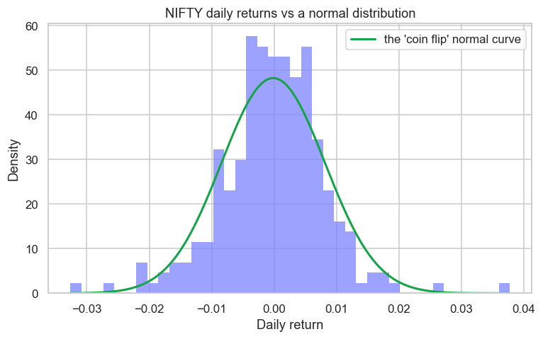
That excess kurtosis of 2.55 is the number that matters. Zero would mean a perfect bell curve. A positive value means fat tails: those big up and down days - the gaps, the circuit-hitting sessions - happen far more often than a normal coin-flip world allows. This single fact quietly breaks half of classical finance, and it's why a quant never assumes the market is "normal." You can see it in the chart: real returns pile up taller in the middle and stretch out further at the edges than the green curve permits.

How a quant actually works

So if not gut feeling, then what? Every quant - from a college grad to a fund running thousands of crores - runs the same loop. It is the scientific method, pointed at markets:

It starts with a hunch ("stocks that gap up keep rising") - the same raw idea any trader has. The quant's difference is what comes next: turn it into a precise hypothesis you can be wrong about, gather honest data, test it without cheating, and ask whether there's a real edge. Most ideas die at the test - and that's not failure, that's the filter working. The few that survive become strategies. You'll run this exact loop, end to end, in the final chapter.

The four kinds of quant

"Quant" isn't one job. In the Indian market you'll find broadly four homes, and they want different things from you:

• Sell-side (broker/bank) quants build pricing models and tools - think the desk that prices exotic options or builds the risk engine.
• Buy-side (AMC / hedge fund / PMS) quants hunt for alpha - the signals that actually make money - and run systematic portfolios.
• Proprietary (prop) trading quants trade the firm's own capital, often intraday, where execution and risk are everything.
• High-frequency (HFT) quants live in microseconds, colocated next to the NSE engine, where the edge is speed and microstructure.

This course leans toward the buy-side and prop mindset - finding and validating edges - because that's what most people mean by "becoming a quant," and it's the most accessible path with a tool like OpenAlgo.

The quant's toolkit

Strip away the mystique and a working quant stands on four legs, each a module of this course:

1. Market structure - knowing how prices are really formed, not just how charts look (Modules A-B).
2. The mathematics of markets - probability, statistics, time series - explained here in plain words, never dropped on you (Modules C-E).
3. Code - to fetch data, test ideas and execute. You'll use Python and the OpenAlgo SDK; if you've done the /python course, you're ready.
4. Skepticism - the hardest and most valuable leg: the discipline to assume your beautiful backtest is wrong until it proves otherwise (Module H).

Try it yourself

• Re-run the first example on BANKNIFTY (exchange NSE_INDEX). Is Bank Nifty's split of up vs down days different from Nifty's? Is it more or less of a coin flip?
• Change the history window in the distribution example from 365 days to 1000. Do the tails get fatter or thinner with more data?
• Pick a belief you hold about the market ("Mondays are weak", "gap-ups fade"). Write it as a one-sentence hypothesis you could actually test. You've just taken the first step of the research loop.

Recap

• A quant is a trader who replaces opinion with measurement, then tests whether the measurement is real or just luck.
• Even a six-line count of Nifty's up/down days reveals what a feeling hides - the edge is often in the shape of moves, not in being right more often.
• Real market returns have fat tails (Nifty's excess kurtosis ≈ 2.5) - the market is not a coin flip, and assuming it is breaks classical finance.
• Every quant runs the same research loop: hunch → hypothesis → data → test → edge, iterating because most ideas fail.
• Quants work across sell-side, buy-side, prop and HFT; this course builds the buy-side/prop skill of finding and validating edges.
• The toolkit is four legs - market structure, maths, code, skepticism - and you can start with just curiosity and basic Python.

Next, we unfold the playing field itself: the map of Indian markets - NSE and BSE, the indices that everyone watches, and the cast of participants whose orders actually move the price.