Time-Series Models (AR, MA, ARIMA)

Module C left us with a hard truth: returns behave like a random walk, their direction barely predictable. So why does an entire field - time-series analysis - exist to model series that depend on their own past? Because "barely predictable" isn't "never," and because the same tools that disappoint on returns become powerful the moment you point them at the right target. This chapter introduces the classic models - AR, MA, ARIMA - honestly: what they are, why they underwhelm on returns, and where they genuinely shine.

AR, MA and ARIMA in plain words

The whole family is built from two simple ideas about how today depends on the past:

• AR (autoregressive) - today is partly a slice of yesterday's value. The weight is φ; if it's large, the series has momentum or mean-reversion you can lean on.
• MA (moving average) - today is partly a slice of yesterday's shock (the surprise, the error). The weight is θ.
• I (integrated) - the "difference it first" step that turns a non-stationary series (like price) into a stationary one (like returns) before modelling.

Stack them and you get ARIMA(p, d, q) - p AR terms, d differences, q MA terms. It's the workhorse of classical time-series forecasting, and learning to read those three numbers tells you exactly what a model is assuming.

Fitting ARIMA to Nifty returns

Theory is cheap; let's fit one and read the verdict:

# Fit an ARIMA model to Nifty returns and forecast - and see how little it can say.
import os
import warnings
from datetime import datetime

from openalgo import api
from statsmodels.tsa.arima.model import ARIMA

warnings.filterwarnings("ignore")

client = api(
    api_key=os.getenv("OPENALGO_API_KEY", "your_api_key_here"),
    host=os.getenv("OPENALGO_HOST", "http://127.0.0.1:5000"),
)

end = datetime.now().strftime("%Y-%m-%d")
r = client.history(symbol="NIFTY", exchange="NSE_INDEX", interval="D",
                   start_date="2021-01-01", end_date=end)["close"].pct_change().dropna() * 100

# ARIMA(1,0,1): today's return from 1 past return (AR) + 1 past shock (MA).
model = ARIMA(r.values, order=(1, 0, 1)).fit()
ar = model.arparams[0] if len(model.arparams) else 0.0
ma = model.maparams[0] if len(model.maparams) else 0.0

print("ARIMA(1,0,1) fitted to Nifty daily returns:")
print(f"  AR coefficient (weight on yesterday's return): {ar:+.3f}")
print(f"  MA coefficient (weight on yesterday's shock)  : {ma:+.3f}")
print(f"\n5-day forecast (%): {[round(float(x), 3) for x in model.forecast(5)]}")
print(f"Mean daily return  : {r.mean():.3f}%")
print("\nThe coefficients are tiny and the forecast collapses to the mean - returns barely autocorrelate.")

ARIMA(1,0,1) fitted to Nifty daily returns:
  AR coefficient (weight on yesterday's return): +0.002
  MA coefficient (weight on yesterday's shock)  : +0.002

5-day forecast (%): [0.047, 0.044, 0.044, 0.044, 0.044]
Mean daily return  : 0.044%

The coefficients are tiny and the forecast collapses to the mean - returns barely autocorrelate.

Both coefficients come out tiny - around 0.002 - meaning yesterday's return and yesterday's shock each carry almost no weight for today. And watch the forecast: it takes one small step and then collapses to the mean and stays there. That's the model honestly telling you it has nothing to say about direction. It isn't broken - it's correctly reporting that Nifty returns are close to white noise, exactly as the random walk predicted.

The diagnostic: ACF and PACF

How would you choose the orders p and q? With two diagnostic plots - the autocorrelation function (ACF) and partial autocorrelation function (PACF) - which reveal at which lags a series carries memory:

Copy

# ACF and PACF: the diagnostic that reveals how little structure returns carry.
import os
from datetime import datetime
from pathlib import Path

import matplotlib

matplotlib.use("Agg")
import matplotlib.pyplot as plt
import seaborn as sns
from openalgo import api
from statsmodels.graphics.tsaplots import plot_acf, plot_pacf

client = api(
    api_key=os.getenv("OPENALGO_API_KEY", "your_api_key_here"),
    host=os.getenv("OPENALGO_HOST", "http://127.0.0.1:5000"),
)

end = datetime.now().strftime("%Y-%m-%d")
r = client.history(symbol="NIFTY", exchange="NSE_INDEX", interval="D",
                   start_date="2021-01-01", end_date=end)["close"].pct_change().dropna()

sns.set_theme(style="whitegrid")
fig, ax = plt.subplots(1, 2, figsize=(10, 4))
plot_acf(r, lags=20, ax=ax[0], color="#7c83ff", vlines_kwargs={"colors": "#7c83ff"})
ax[0].set_title("ACF of returns - bars inside the band = no memory")
plot_pacf(r, lags=20, ax=ax[1], method="ywm", color="#16a34a", vlines_kwargs={"colors": "#16a34a"})
ax[1].set_title("PACF of returns - almost no usable structure")

fig.tight_layout()
out = Path(__file__).with_suffix(".png")
plt.savefig(out, dpi=110, bbox_inches="tight")
inside = (abs(r.autocorr(1)) < 2 / len(r) ** 0.5)
print(f"Lag-1 autocorrelation {r.autocorr(1):.3f} (inside 95% band: {inside}). Returns are near white noise. Saved {out.name}")

Live output

Lag-1 autocorrelation 0.004 (inside 95% band: True). Returns are near white noise. Saved 02_acf_pacf.png

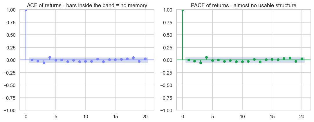
Read the bars against the shaded confidence band: a bar poking outside the band means real structure at that lag; a bar inside means noise. For Nifty returns, almost everything sits inside the band - there's no usable signal at any lag. The diagnostic isn't failing; it's confirming there's nothing to model. On a series with genuine memory, these plots would light up and tell you precisely which AR and MA terms to include.

So are these models useless?

Not at all - you're just pointing them at the wrong target. ARIMA underwhelms on returns because returns are nearly memoryless. But aim the very same machinery at series that genuinely do remember their past, and it comes alive:

• Volatility clusters and is highly autocorrelated - and modelling it is the entire next chapter (GARCH is a close cousin of ARIMA for variance).
• Spreads between cointegrated assets are stationary and mean-reverting - perfect ARIMA territory, and the engine of pairs trading (Chapter 17).
• Macro and fundamental series - rates, inflation, volumes - carry real time structure.

What's truly predictable

So the chapter's quiet lesson, echoing Chapter 11: direction is nearly unforecastable, but the market is not all noise. Its volatility has memory, its relationships mean-revert, and its structure leaves footprints. The rest of Module D builds models for exactly those predictable corners - starting, next, with the one every options trader cares about: volatility itself.

Try it yourself

• Fit ARIMA(1,0,1) to the absolute returns (|r|) instead of returns. Are the coefficients bigger now? (Volatility has the memory returns lack.)
• Run the ACF/PACF on a cointegrated spread (HDFCBANK − ICICIBANK). Do bars poke outside the band, hinting at real structure?
• Increase the ARIMA order to (5,0,5) on returns. Does the forecast get any less flat, or does added complexity just fit noise?

Recap

• AR models today from past values, MA from past shocks, and I differences a non-stationary series first - combined as ARIMA(p, d, q).
• Fitted to Nifty returns, ARIMA gives near-zero coefficients and a forecast that collapses to the mean - returns are close to white noise.
• The ACF and PACF plots diagnose where a series has memory; for returns, nearly everything sits inside the confidence band - no structure to model.
• The models aren't useless - they're powerful on series that genuinely remember their past: volatility, spreads, and macro series, not raw returns.
• The real skill is choosing the right target - modelling what has memory, not forcing a model onto noise.

The first series with real memory is volatility - it clusters, it persists, and unlike returns, it can genuinely be forecast. Next we build the model that does it: GARCH.