Portfolio Construction, Risk Models, VaR and Stress

A single brilliant signal is a lottery ticket; a well-built book is a machine. The whole course so far has hunted edges one at a time - a momentum tilt here, a mean-reversion in BANKNIFTY there, a vol-selling overlay on the side. This chapter, the closer of Module H, is where they all arrive at the same desk and become one risk-managed portfolio. The job has three parts that nobody gets to skip: decide how to weight many positions so the whole is safer than the sum, decide how much to bet in total, and decide how to survive the rare day the bell curve swore was impossible. Get the weighting and sizing right and a modest edge compounds for decades. Get the tail wrong once and none of the rest matters.

From many signals to one book

Start with the one fact that makes portfolios worth building. A portfolio's return is just the weighted average of its holdings' returns. But its risk is not the weighted average of their risks - it depends on how the assets move relative to each other. The mathematical name for "how they move together" is covariance (standardised, it is correlation), and it is the single most important quantity in portfolio construction. Two names that zig and zag at different times partly cancel, so the blend is calmer than either alone.

That is not a theory you have to take on faith - it is measurable on real money. Take five very different NSE names, weight them by risk, and the portfolio's annualised volatility lands at 14.1%, lower than any of the individual stocks that make it up. You gave up nothing in expected return; you simply combined imperfectly correlated assets and let the risk partly cancel. That free reduction in risk is, in the famous phrase, the only free lunch in finance, and it is why no serious quant ever bets the whole book on one name.

Mean-variance, and why it breaks live

If diversification is good, what is the best mix? Harry Markowitz answered this in 1952 and won a Nobel for it. Mean-variance optimisation takes your estimated expected returns and the covariance matrix and solves directly for the weights that maximise return for a given risk, tracing out the efficient frontier - the hard upper-left edge of all achievable portfolios, where each point gives the most return possible for its volatility. The single best point on it is the maximum-Sharpe portfolio. It is the founding image of modern finance, and in its raw form professionals almost never use it. Here is why.

Mean-variance optimisation is an error-maximiser. It needs two inputs - expected returns and covariances - and both are estimated from a finite, noisy past. The optimiser, hunting for the best blend, gleefully pours capital into whichever asset's return was over-estimated by luck, producing portfolios that are wildly concentrated, unstable, and that lurch when you add a single day of data. The maths is flawless; the inputs are guesses, and the machine magnifies every guessing error.

Real desks keep the insight of portfolio theory while taming its fragility. Equal weight is astonishingly hard to beat because it makes no fragile return forecast at all. Shrinkage pulls noisy estimates toward a sensible prior (Ledoit-Wolf for the covariance matrix) so the optimiser cannot chase noise. Constraints cap position sizes and ban shorts so it cannot make insane bets. And Black-Litterman starts from the market's equilibrium weights and tilts gently toward your views in proportion to your confidence, sidestepping the error-maximisation entirely.

Sizing the book: risk parity, volatility targeting and Kelly

The most useful idea between naive equal weight and fragile optimisation is risk parity: weight each holding so that every one contributes equal risk to the portfolio, not equal capital. A volatile name gets a smaller rupee weight, a calm one a larger weight, so no single position quietly dominates the book's swings. The clean first approximation is inverse-volatility weighting - divide one by each asset's volatility and normalise. That is exactly what the example below does, and it is why TATASTEEL (the wildest of the five) gets the smallest slice and the steadier banks and ITC get the largest.

# Risk-parity weights from real NSE returns, then the book's 1-day 95% VaR and CVaR.
import os
from datetime import datetime, timedelta

import numpy as np
import pandas as pd
from openalgo import api

client = api(
    api_key=os.getenv("OPENALGO_API_KEY", "your_api_key_here"),
    host=os.getenv("OPENALGO_HOST", "http://127.0.0.1:5000"),
)

end = datetime.now().strftime("%Y-%m-%d")
start = (datetime.now() - timedelta(days=1095)).strftime("%Y-%m-%d")
syms = ["RELIANCE", "HDFCBANK", "INFY", "ITC", "TATASTEEL"]

rets = pd.DataFrame({s: client.history(symbol=s, exchange="NSE", interval="D",
                                       start_date=start, end_date=end)["close"].pct_change()
                     for s in syms}).dropna()

# Risk parity (inverse-volatility): each name contributes roughly equal risk,
# so a calm stock gets a bigger rupee weight than a wild one.
vol = rets.std()
w = (1 / vol) / (1 / vol).sum()

port = rets @ w                      # daily portfolio returns
ann_vol = port.std() * np.sqrt(252) * 100

# Historical 1-day 95% VaR / CVaR: VaR is the 5th-percentile loss;
# CVaR (expected shortfall) is the average loss across the whole tail beyond it.
cut = np.percentile(port, 5)
var95 = -cut * 100
cvar95 = -port[port <= cut].mean() * 100
worst = -port.min() * 100

print("Risk-parity (inverse-vol) weights:")
for s in syms:
    print(f"  {s:10s}: {w[s] * 100:5.1f}%")
print(f"\nPortfolio annualised vol  : {ann_vol:.1f}%")
print(f"Historical 1-day 95% VaR  : -{var95:.2f}%")
print(f"Historical 1-day 95% CVaR : -{cvar95:.2f}%")
print(f"Worst single day in window: -{worst:.2f}%")
print(f"\nOn 19 days in 20 the book loses under {var95:.2f}%; when it breaches, it averages {cvar95:.2f}%.")

Risk-parity (inverse-vol) weights:
  RELIANCE  :  21.0%
  HDFCBANK  :  22.4%
  INFY      :  17.4%
  ITC       :  23.3%
  TATASTEEL :  15.8%

Portfolio annualised vol  : 14.1%
Historical 1-day 95% VaR  : -1.42%
Historical 1-day 95% CVaR : -2.04%
Worst single day in window: -5.24%

On 19 days in 20 the book loses under 1.42%; when it breaches, it averages 2.04%.

The weights come out RELIANCE 21.0%, HDFCBANK 22.4%, INFY 17.4%, ITC 23.3% and TATASTEEL 15.8% - and the resulting book sits at 14.1% annualised volatility. The same trick applied through time is volatility targeting: pick a target risk level, say 12% annualised, and scale total exposure inversely to recent realised volatility - smaller when markets are wild, larger when they are calm - so the book's risk stays roughly constant even as conditions swing. It automatically pulls you out of harm's way exactly when volatility, and danger, spikes.

That decides relative weights and steady risk. One question still decides whether you compound or go broke: how much total capital do you bet? The growth-optimal answer is the Kelly criterion, derived by John Kelly at Bell Labs in 1956. For a return stream the Kelly fraction is, intuitively, your edge divided by your variance. Bet that and you maximise the long-run growth rate of capital. Bet more and - this is the part that humbles aggressive traders - you grow slower and eventually to ruin. Past the peak, betting more with a winning edge makes you poorer.

Factor risk models

Risk parity treats each name as a risk unit, but names are not independent bets - RELIANCE, HDFCBANK and INFY all load on the broad market, and many of your signals are secretly the same trade. A factor risk model decomposes each asset's risk into a handful of common drivers (the market, size, value, momentum, quality, low-volatility, plus sectors) and a small idiosyncratic remainder. The model rebuilds the covariance matrix as factor exposures times factor covariances, which is both far more stable to estimate than a raw stock-by-stock matrix and far more honest about concentration. Two positions that look diversified by name can carry one giant hidden bet - long momentum, short value, or simply 90% market beta. The point of a factor model is to see that bet before the market shows it to you, and to set limits on factor exposure rather than only on single stocks.

VaR, expected shortfall and the tail you actually die in

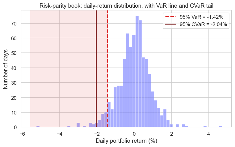
Accounts do not die in the normal world; they die in the tail, on the one day the model called impossible. The industry's standard tail metric is Value at Risk (VaR): the loss you will not exceed at some confidence, over some horizon. For the risk-parity book above, the historical 1-day 95% VaR is -1.42% - meaning on 19 days in 20 the book loses less than 1.42%. Useful shorthand for a normal bad day. But it hides two things that have killed real institutions.

First, VaR is silent about how bad it gets beyond the line. The fix is expected shortfall, or CVaR (conditional VaR): instead of the threshold, average the loss across the entire tail beyond it. For this book CVaR comes out at -2.04%, noticeably worse than the -1.42% VaR, because it counts the brutal far-tail days the threshold ignores. Second, the worst single day in the three-year window was -5.24% - and that window does not even contain a genuine crisis. The picture below shades the tail so you can see VaR as a line and CVaR as the average of everything beyond it.

Copy

# The risk-parity book's daily-return distribution with the 95% VaR line and CVaR tail marked.
import os
from datetime import datetime, timedelta
from pathlib import Path

import matplotlib

matplotlib.use("Agg")
import matplotlib.pyplot as plt
import numpy as np
import pandas as pd
import seaborn as sns
from openalgo import api

client = api(
    api_key=os.getenv("OPENALGO_API_KEY", "your_api_key_here"),
    host=os.getenv("OPENALGO_HOST", "http://127.0.0.1:5000"),
)

end = datetime.now().strftime("%Y-%m-%d")
start = (datetime.now() - timedelta(days=1095)).strftime("%Y-%m-%d")
syms = ["RELIANCE", "HDFCBANK", "INFY", "ITC", "TATASTEEL"]
rets = pd.DataFrame({s: client.history(symbol=s, exchange="NSE", interval="D",
                                       start_date=start, end_date=end)["close"].pct_change()
                     for s in syms}).dropna()

vol = rets.std()
w = (1 / vol) / (1 / vol).sum()
port = (rets @ w) * 100              # daily portfolio returns, in percent

var95 = np.percentile(port, 5)       # threshold loss (negative)
cvar95 = port[port <= var95].mean()  # average loss across the tail

sns.set_theme(style="whitegrid")
fig, ax = plt.subplots(figsize=(8, 4.5))
sns.histplot(port, bins=60, color="#7c83ff", alpha=0.65, edgecolor="white", linewidth=0.3, ax=ax)
ax.axvspan(port.min() - 0.3, var95, color="#dc2626", alpha=0.10)
ax.axvline(var95, color="#dc2626", lw=2, ls="--", label=f"95% VaR = {var95:.2f}%")
ax.axvline(cvar95, color="#7c1d1d", lw=2, label=f"95% CVaR = {cvar95:.2f}%")
ax.set_title("Risk-parity book: daily-return distribution, with VaR line and CVaR tail")
ax.set_xlabel("Daily portfolio return (%)")
ax.set_ylabel("Number of days")
ax.legend()

out = Path(__file__).with_suffix(".png")
plt.savefig(out, dpi=110, bbox_inches="tight")
print(f"VaR {var95:.2f}%, CVaR {cvar95:.2f}%, worst day {port.min():.2f}%. Saved {out.name}")

Live output

VaR -1.42%, CVaR -2.04%, worst day -5.24%. Saved 02_var_distribution.png

Stress testing and the road ahead

History only contains the shocks that happened. Our three-year sample tops out at a -5.24% day, yet the COVID crash of March 2020 delivered a -13% day and a roughly -38% drawdown, and demonetisation and election-result days have swung violently before. Stress testing asks about the shocks your sample never saw: what does the book lose if NIFTY gaps down 10% overnight, if volatility triples, if liquidity vanishes and correlations all rush to one? Rather than trusting a statistical model, you impose specific brutal scenarios and read the damage directly. A quant who has stress-tested for a -15% gap is not surprised when one arrives, and crucially is not over-sized into it.

That completes Module H. We can now take many edges and build a single portfolio, size it so a good year does not become the year that ruins us, and guard the tail that statistics alone will always under-state. Everything until now has been research and construction. Module I is where it goes live: the research-to-production pipeline, live system design, monitoring and reconciliation, and the discipline of running real capital under real regulation.