Why Market Microstructure Matters

Pull up any chart and you see a clean line of prices marching left to right, one crisp number per bar. That line is a comforting fiction. It is a museum of prices that have already happened - the last handshake recorded at each instant - and not one of them is a price you can trade at right now. The moment you try to buy, you discover the secret every market hides in plain sight: there is no single price. There is a price to buy and a slightly worse price to sell, a queue you must join or jump, and a cost you forfeit before the market has moved a single paisa in your favour. Market microstructure is the study of exactly this machinery - how resting orders turn into trades, and what that turning costs you. It is where most retail edges, beautiful on a backtest, quietly bleed to death. This module is about learning to see the cost before it sees you.

The price on the chart is not the price you get

Microstructure is the close-up view of the market: not where price is going over the next month, but how a single trade actually gets done in the next second. The first thing it forces you to admit is that the chart shows one number while the market quotes two.

At any instant the order book holds a best bid - the highest price a resting buyer will pay - and a best ask, the lowest price a resting seller will accept. You sell into the bid; you buy from the ask. The gap between them is the bid-ask spread, and it is the single most important number in this whole module. The chart's last-traded line usually sits somewhere between the two, but you can never trade at the chart. You trade at the bid or the ask, whichever is worse for you.

We measure that gap in basis points (bps), where one basis point is one hundredth of a percent, or one ten-thousandth of the price. Basis points let us compare a spread on a Rs 6,500 commodity with a spread on a Rs 1,300 stock on the same scale: it is the cost as a fraction of what you are trading, not in rupees. The quoted spread translates directly into the gap between the quoted price (what the chart and the ticker show) and the effective price (what you genuinely fill at). Cross the spread to trade immediately and you are a liquidity taker; you pay that gap for the privilege of certainty.

The spread is a cost you pay up front

Theory is cheap; let us price a real spread. The example below opens an MCX crude future - commodities trade into the night, so there is genuine activity when NSE and BSE are dark - and converts its spread into rupees, basis points and the cost of a full round trip.

# The gap between the chart price and your fill: the spread in rupees, basis points and round-trip cost.
import os

from openalgo import api

client = api(
    api_key=os.getenv("OPENALGO_API_KEY", "your_api_key_here"),
    host=os.getenv("OPENALGO_HOST", "http://127.0.0.1:5000"),
)

# A near-month MCX crude future: deeply liquid, and it trades into the night.
SYMBOL, EXCHANGE = "CRUDEOIL20JUL26FUT", "MCX"
tick = client.symbol(symbol=SYMBOL, exchange=EXCHANGE)["data"]["tick_size"]

d = client.depth(symbol=SYMBOL, exchange=EXCHANGE)["data"]
bid, ask = d["bids"][0]["price"], d["asks"][0]["price"]

if bid > 0 and ask > 0:
    # Live book: the spread is the real distance between best bid and best ask.
    source = "live L5 book"
    spread = ask - bid
    mid = (bid + ask) / 2.0
else:
    # Book is shut, so we cannot see it. Proxy the spread by how far price
    # travels inside a typical one-minute bar (an honest upper bracket).
    source = "range proxy (book shut)"
    df = client.history(symbol=SYMBOL, exchange=EXCHANGE, interval="1m",
                        start_date="2026-06-25", end_date="2026-06-27")
    df = df[df["volume"] > 0]
    spread = float((df["high"] - df["low"]).median())
    mid = float(df["close"].iloc[-1])

spread_bps = spread / mid * 1e4
floor_bps = tick / mid * 1e4                 # the tightest the spread can ever be: one tick
round_trip = spread_bps / 1e4 * 100000       # cross in at ask, out at bid, on Rs 1,00,000 traded

print(f"{SYMBOL}  ({source})")
print(f"Mid ~ {mid:.1f}   tick size Rs {tick:g}  ({floor_bps:.1f} bps floor)")
print(f"Spread        Rs {spread:.1f}   =  {spread_bps:.1f} bps of price")
print(f"Round trip    forfeit the full spread in and out  =  Rs {round_trip:.0f} per Rs 1,00,000 traded")

CRUDEOIL20JUL26FUT  (range proxy (book shut))
Mid ~ 6570.0   tick size Rs 1  (1.5 bps floor)
Spread        Rs 6.0   =  9.1 bps of price
Round trip    forfeit the full spread in and out  =  Rs 91 per Rs 1,00,000 traded

On a mid price of about Rs 6,570, the measured spread is roughly Rs 6, or about 9.1 bps of price. (The book was shut at run time, so the script honestly falls back to a per-minute range proxy, an upper bracket on the true quoted spread rather than the live quote.) The tick size is Rs 1, which sets a hard floor of about 1.5 bps - the spread can never be tighter than one tick, no matter how liquid the contract. The number that should sting is the round trip: cross in at the ask and out at the bid and you forfeit the full spread twice, about Rs 91 for every Rs 1,00,000 you turn over. You have paid that before brokerage, before STT, before the market has ticked once. Trade this contract ten times in a day and the spread alone has quietly skimmed nearly Rs 1,000 per lakh of turnover off the top.

This is why the spread, not brokerage, is the cost that decides whether a high-frequency idea is even worth coding. A strategy that nets two basis points per trade is dead on arrival against a nine basis point spread. The faster you trade, the more times a day you pay the spread, and the larger it looms relative to whatever edge you think you have.

Even patient, slow traders pay

The common rebuttal is reasonable: "I hold for weeks, and I use limit orders, so the spread is somebody else's problem." It is not. There are three quiet leaks even the most patient trader cannot fully plug.

First, you still have to get in and out. A position held for a month is still opened and closed by an order that crosses the spread or rests and risks not filling. The cost is amortised over a longer hold, which softens it, but it never reaches zero. Second, limit orders are not free either: rest on the bid and you fill only when someone wants to sell to you, which is disproportionately when they know something you do not. That is adverse selection, and it is the price of the better price. Third, and most brutal, the spread is not a constant. It widens exactly when you most want to trade - on news, at the open, into a fast move - so the cost you budgeted from a calm midday snapshot understates what you actually pay in the moment that matters.

The second example makes that variability visible. It pulls one full session of one-minute bars for RELIANCE and uses the bar range as a cost proxy, minute by minute.

Copy

# Trading cost is not constant: a per-bar spread proxy over one session reveals the intraday U-shape.
import os
from pathlib import Path

import matplotlib

matplotlib.use("Agg")
import matplotlib.dates as mdates
import matplotlib.pyplot as plt
import seaborn as sns
from openalgo import api

client = api(
    api_key=os.getenv("OPENALGO_API_KEY", "your_api_key_here"),
    host=os.getenv("OPENALGO_HOST", "http://127.0.0.1:5000"),
)

SYMBOL, EXCHANGE, DAY = "RELIANCE", "NSE", "2026-06-25"
df = client.history(symbol=SYMBOL, exchange=EXCHANGE, interval="1m",
                    start_date=DAY, end_date=DAY)
df = df[df["volume"] > 0].copy()
df.index = df.index.tz_localize(None)        # show the IST clock on the x-axis

# Per-bar cost proxy: how far price travels inside one minute, in basis points of price.
df["cost_bps"] = (df["high"] - df["low"]) / df["close"] * 1e4
df["smooth"] = df["cost_bps"].rolling(10, min_periods=1).mean()
median = df["cost_bps"].median()

sns.set_theme(style="whitegrid")
fig, ax = plt.subplots(figsize=(9, 4.5))
ax.scatter(df.index, df["cost_bps"], s=6, color="#c9ccd6", alpha=0.5, label="per-minute proxy")
ax.plot(df.index, df["smooth"], color="#7c83ff", lw=2, label="10-minute average")
ax.axhline(median, color="#16a34a", ls="--", lw=1, label=f"median {median:.1f} bps")
ax.set_title(f"{SYMBOL} {DAY} - cost of crossing the spread, by minute")
ax.set_xlabel("Time of day (IST)")
ax.set_ylabel("Cost proxy (bps of price)")
ax.xaxis.set_major_formatter(mdates.DateFormatter("%H:%M"))
ax.legend(loc="upper center", ncol=3, frameon=False)

out = Path(__file__).with_suffix(".png")
plt.savefig(out, dpi=110, bbox_inches="tight")

open15 = df["cost_bps"].iloc[:15].mean()
midday = df["cost_bps"].between_time("12:00", "13:00").mean()
close15 = df["cost_bps"].iloc[-15:].mean()
print(f"{SYMBOL} {DAY}: open {open15:.1f} bps, midday {midday:.1f} bps, close {close15:.1f} bps "
      f"- cost is widest at the open. Saved {out.name}")

Live output

RELIANCE 2026-06-25: open 12.2 bps, midday 5.6 bps, close 6.4 bps - cost is widest at the open. Saved 02_intraday_cost.png

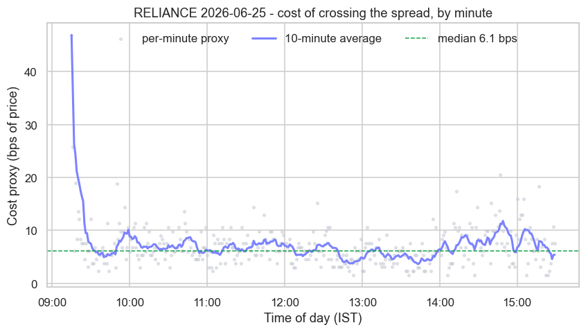
The shape is the lesson. The cost proxy averages about 12.2 bps in the opening minutes, falls to roughly 5.6 bps through midday, and sits near 6.4 bps into the close. The most expensive time to trade is the opening bell - more than double the midday cost - which is precisely when retail momentum traders feel the most urgency to act on the overnight news and the gap. You pay the widest spread at the exact moment you feel most compelled to cross it.

The deeper point is that the spread is the market's price for liquidity, and that price is set by the order book second to second. Microstructure is simply the discipline of reading and respecting that price. Ignore it and your backtest, computed on mid prices or close prices that nobody can trade, will promise an edge the live market never delivers.

A map of Module C

Everything ahead in this module is a sharper lens on the machinery you just met. Here is the path:

• ch18 to ch20 - the order book and matching. The limit order book in full, the order types and lifecycle you will actually send, and price-time priority - why being early in the queue at a price has real monetary value.
• ch21 to ch24 - the structure of the trading day. Sessions from pre-open to close, the call and closing auctions, circuit breakers and price bands, and the special bulk and block deal windows where large size changes hands.
• ch25 to ch27 - the economics of liquidity. Spread and depth measured properly, impact cost and transaction cost analysis (how your own order moves the price), and what open interest, volume and order flow reveal about pressure.
• ch28 - the short side. Short selling, the securities lending and borrowing market, and the borrowing mechanics a market-neutral book lives on.

You now know the uncomfortable truth that the chart lies by omission: it shows the price of the last trade, never the price of your trade. The rest of this module hands you the tools to see both. We start at the source of every price in the next chapter, by opening the limit order book itself and reading the resting bids and asks that decide what your fill will be.