Distributions, Fat Tails and Extreme Moves

In the last chapter we met the fat tails of returns as one of four stylized facts and moved on. Now we stop and stare at them, because the tail is where careers end. Almost every blow-up in trading history - leveraged funds, options sellers, "market-neutral" books - died the same way: someone built risk on the normal distribution, the comforting bell curve, and the market handed them a day the bell swore was impossible. The normal is a beautiful model of the calm centre of returns and a dangerous lie about their edges. This chapter is about the edges: how to measure them, how to model them, and how to size a position so a single violent day does not take you out of the game.

The bell curve's broken promise

The normal distribution makes a precise promise. Once you know the mean and the standard deviation - call it sigma, the typical size of a daily move - it claims to know exactly how often every size of move occurs. A move beyond 3 sigma should happen about once in 740 days. A move beyond 4 sigma should happen once in roughly 16,000 days, about once in 63 years of trading. The promise is testable, so let us test it on eleven years of NIFTY:

# How often NIFTY breaches 4 sigma - the normal's prediction versus reality.
import os
from datetime import datetime

import numpy as np
from openalgo import api
from scipy import stats

client = api(
    api_key=os.getenv("OPENALGO_API_KEY", "your_api_key_here"),
    host=os.getenv("OPENALGO_HOST", "http://127.0.0.1:5000"),
)

end = datetime.now().strftime("%Y-%m-%d")
df = client.history(symbol="NIFTY", exchange="NSE_INDEX", interval="D",
                    start_date="2015-01-01", end_date=end)
r = np.log(df["close"] / df["close"].shift(1)).dropna()
n = len(r)
sigma = r.std()

# Shape of the distribution
skew = stats.skew(r)
ex_kurt = stats.kurtosis(r)  # excess kurtosis (normal = 0)

# Days beyond 4 standard deviations, observed vs what a normal predicts
z = (r - r.mean()) / sigma
beyond4 = int((z.abs() > 4).sum())
p_normal = 2 * stats.norm.sf(4)          # P(|Z| > 4) under a normal
expected4 = n * p_normal

worst = r.min()
print(f"NIFTY daily log returns since 2015: {n} days, sigma {sigma*100:.2f}%")
print(f"Skew {skew:.2f}, excess kurtosis {ex_kurt:.2f} (normal = 0)")
print(f"Beyond-4-sigma days: observed {beyond4}, a normal predicts {expected4:.2f}")
print(f"Reality delivers {beyond4/expected4:.0f}x the normal count. "
      f"Worst single day: {worst*100:.1f}%")

NIFTY daily log returns since 2015: 2843 days, sigma 1.03%
Skew -1.31, excess kurtosis 19.60 (normal = 0)
Beyond-4-sigma days: observed 16, a normal predicts 0.18
Reality delivers 89x the normal count. Worst single day: -13.9%

The result is not a rounding error - it is a different universe. Across 2843 trading days since 2015, with a daily sigma of 1.03%, a normal distribution predicts 0.18 days beyond 4 sigma. NIFTY delivered 16. That is roughly 89 times the textbook count, and it includes a single day that fell 13.9%. Measured in sigmas, a 13.9% drop is more than thirteen standard deviations. Under the normal, a thirteen-sigma day has a probability so small you would not expect to see one in billions of years of trading. The market produced it in March 2020 anyway.

Skew and kurtosis: shape beyond mean and variance

Mean and variance describe where a distribution sits and how wide it is. They say nothing about its shape. Two more numbers - the third and fourth standardised moments - capture the part that matters for risk.

Skewness measures asymmetry. A negative skew means the left tail is longer than the right: crashes are sharper than rallies. NIFTY's daily skew comes out at -1.31, firmly negative, which is the quant signature of equity indices everywhere. Markets take the stairs up and the elevator down. The down days are not just more frequent in the tail, they are individually larger, and a risk model that assumes symmetry will systematically under-price exactly the move that hurts.

Kurtosis measures tail heaviness - how much of the action hides in rare extremes. A normal has an excess kurtosis of 0. NIFTY's daily returns since 2015 show an excess kurtosis of 19.60. In the previous chapter the same statistic on a shorter, post-2021 window read about 3.7. The jump is not a contradiction; it is the whole lesson. Add the March 2020 window back in and one observation - the 13.9% day - drags the fourth moment up enormously.

The Student-t and the power law in the tail

If the normal is the wrong shape, what is the right one? The workhorse replacement is the Student-t distribution. It has the same bell shape but one extra knob, the degrees of freedom (written nu), that controls tail weight. A high nu is almost normal; a low nu has heavy tails. Fit a t to standardised NIFTY returns and plot it against the normal:

Copy

# QQ-plot of NIFTY returns: a fitted normal abandons the tails, a Student-t hugs them.
import os
from datetime import datetime
from pathlib import Path

import matplotlib

matplotlib.use("Agg")
import matplotlib.pyplot as plt
import numpy as np
import seaborn as sns
from openalgo import api
from scipy import stats

client = api(
    api_key=os.getenv("OPENALGO_API_KEY", "your_api_key_here"),
    host=os.getenv("OPENALGO_HOST", "http://127.0.0.1:5000"),
)

end = datetime.now().strftime("%Y-%m-%d")
df = client.history(symbol="NIFTY", exchange="NSE_INDEX", interval="D",
                    start_date="2015-01-01", end_date=end)
r = np.log(df["close"] / df["close"].shift(1)).dropna()

# Fit a Student-t to the standardised returns; estimate its tail-heaviness (df)
zr = (r - r.mean()) / r.std()
nu, _, _ = stats.t.fit(zr, floc=0)            # nu = degrees of freedom (lower = fatter)

sns.set_theme(style="whitegrid")
fig, ax = plt.subplots(1, 2, figsize=(11, 4.6))

# Left: QQ-plot of empirical quantiles vs a fitted normal
osm, osr = stats.probplot(zr, dist="norm", fit=False)
ax[0].scatter(osm, osr, s=10, color="#7c83ff", edgecolor="none")
lim = [min(osm.min(), osr.min()), max(osm.max(), osr.max())]
ax[0].plot(lim, lim, color="#16a34a", lw=2, label="normal reference")
ax[0].set_title("QQ-plot vs normal: tails fly off the line")
ax[0].set_xlabel("normal quantiles")
ax[0].set_ylabel("NIFTY return quantiles")
ax[0].legend(loc="upper left")

# Right: log-density histogram with a fitted normal and a fitted Student-t
sns.histplot(zr, bins=120, stat="density", color="#cdd0ff", edgecolor="none", ax=ax[1])
x = np.linspace(zr.min(), zr.max(), 400)
ax[1].plot(x, stats.norm.pdf(x), color="#16a34a", lw=2, label="fitted normal")
ax[1].plot(x, stats.t.pdf(x, nu), color="#dc2626", lw=2, label=f"fitted t (nu={nu:.1f})")
ax[1].set_yscale("log")
ax[1].set_ylim(1e-4, 1)
ax[1].set_title("Log-density: the t hugs the fat tails")
ax[1].set_xlabel("standardised daily return (sigmas)")
ax[1].legend(loc="upper right")

fig.suptitle("NIFTY daily returns since 2015 - normal versus Student-t", fontsize=13)
fig.tight_layout()
out = Path(__file__).with_suffix(".png")
plt.savefig(out, dpi=110, bbox_inches="tight")
print(f"{len(r)} days. Fitted Student-t df nu={nu:.1f} (fat: a normal is nu=inf). Saved {out.name}")

Live output

2843 days. Fitted Student-t df nu=3.7 (fat: a normal is nu=inf). Saved 02_qqplot_t_vs_normal.png

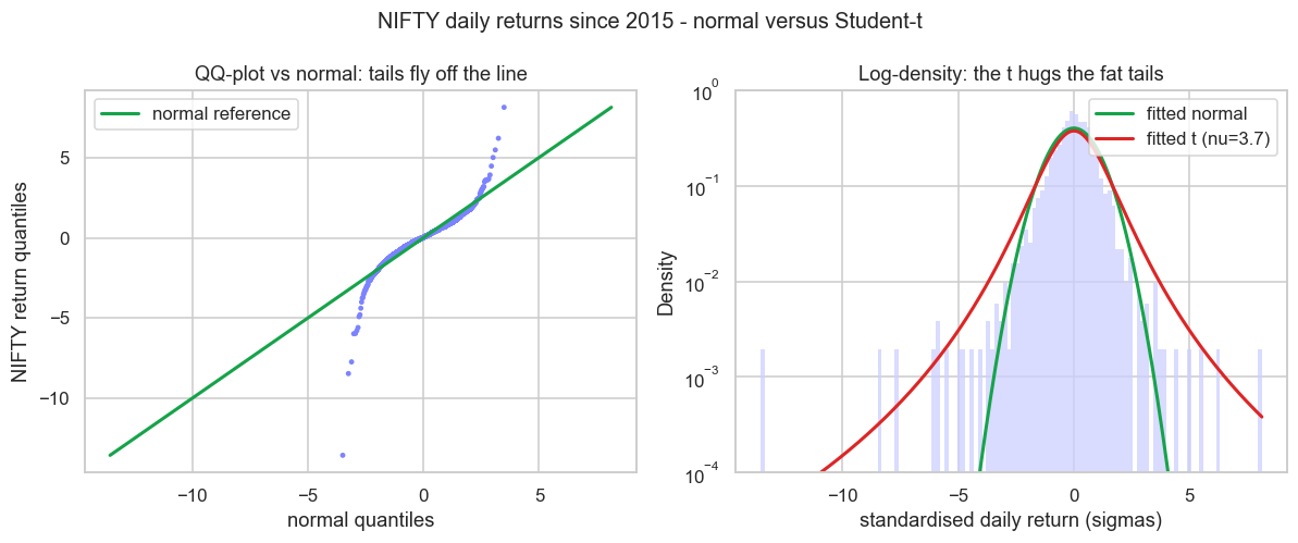
The left panel is a QQ-plot: it lines up the actual return quantiles against what a normal would produce. If returns were normal the dots would sit on the green line. Instead they peel away violently at both ends - the S-shape that screams "fat tails". The right panel, on a log scale, shows the fitted normal (green) plummeting toward zero past 4 sigma while the fitted t with nu near 3.7 (red) stays lifted, tracing the real extreme observations.

That nu near 3.7 carries a deep warning. The t distribution has a finite variance only when nu is above 2, and a finite kurtosis only when nu is above 4. Our fit sits below 4, which means the model that best matches NIFTY has, in theory, an infinite fourth moment. This is the formal face of the power law: deep in the tail the probability of a move of size x decays not exponentially, like the normal, but as a power of x, with an exponent - the tail index - of roughly 3 for equity returns the world over. The famous "inverse cubic law" of returns is exactly this. A tail index near 3 says the variance exists but the kurtosis does not converge, which is precisely why our sample kurtosis was so unstable. The maths and the messy data agree: there is no largest crash you can rule out.

An extreme-value view of Indian crashes

If the tail is its own creature, study it directly. Extreme-value theory (EVT) is the branch of statistics that models the maximum, not the average - the worst day in a block, or every move past a high threshold. It tells you that tail exceedances follow their own universal shape (the generalised Pareto), letting you estimate the size of a once-in-ten-years day from data that does not yet contain one.

The reframe EVT forces is from probability to return period. Instead of "what is the chance of a 6% down day", ask "how often should a 6% down day arrive". For an Indian equity quant the honest answers are sobering. NIFTY has seen demonetisation in 2016, the IL&FS shock in 2018, the COVID waterfall in 2020, and assorted budget-day and global-risk air-pockets - clusters of extreme days that no smooth bell curve would ever generate. And note that fat tails interact with volatility clustering from the previous chapter: extreme days do not arrive alone, they come in storms, which makes the realised loss over a bad week worse still than the single-day tail suggests.

Sizing for the tail you cannot see

All of this is academic until it touches your position size, where it becomes the difference between surviving and not. The core mistake is sizing off sigma. A risk budget that says "lose at most 2% on a 4-sigma day" sounds prudent and is quietly suicidal, because for NIFTY the real bad day is not 4 sigma, it is more than 13. If you set leverage so that a normal-implied worst case is tolerable, the genuine worst case is several times larger and it arrives far more often than the model claims.

A few rules follow directly from fat tails:

• Size to the historical worst day, not to sigma. Before taking leverage, ask what a repeat of the worst day in your data does to your equity. If the answer is "ruin", you are too big, whatever your sigma-based value-at-risk says.
• Haircut the Kelly bet. The Kelly criterion assumes you know the return distribution. Under fat tails that assumption fails on the side that matters, so practitioners run a fraction of full Kelly - half or less - precisely to buy a margin against the tail they cannot measure. We build this properly in Chapter 72.
• Lean on what is predictable. You cannot predict the next crash, but volatility clusters, so scaling exposure down when realised volatility rises - the GARCH machinery of Chapter 42 - removes part of the tail before it hits.
• Respect the asymmetry. Negative skew means your hedges belong on the downside. Selling naked options or shorting volatility harvests a small premium most days and pays it all back, with interest, on the 13-sigma day.

Recap

• The normal distribution fits the body of returns and badly understates the tails: NIFTY since 2015 produced 16 days beyond 4 sigma against a normal prediction of 0.18, including a 13.9% day worth more than thirteen sigma.
• Skewness (NIFTY about -1.31) captures the down-elevator asymmetry; kurtosis (excess 19.60) captures tail heaviness, and it is unstable because one crash dominates it.
• The Student-t fits returns with degrees of freedom near 3.7, below the threshold where kurtosis is even finite - the signature of a power-law tail with index around 3, the inverse cubic law.
• Extreme-value theory models the tail on its own terms and reframes risk as a return period; fat tails plus volatility clustering mean extremes arrive in storms.
• Size for the tail: budget to the worst historical day rather than to sigma, run fractional Kelly, scale down when volatility rises, and never sell the tail you cannot price.

We now respect the distribution of a single asset's returns. Next we widen the lens to many assets at once - the linear algebra, covariance and principal components that let a quant reason about a whole portfolio of fat-tailed instruments together.