Cointegration and Pairs Trading

Two stocks can shadow each other for years and still betray you. Plot HDFC Bank against ICICI Bank and the lines look like twins, rising and falling together with a correlation of 0.78. Yet run the one test that actually matters and the pair falls apart - their gap is free to wander off and never come home. Meanwhile a less obvious pairing, Kotak Mahindra Bank against HDFC Bank, barely 0.72 correlated, turns out to be welded at the hip - its spread snaps back to fair value again and again. That distance between looking related and being tethered is the whole edge of pairs trading, and the tool that separates the two is cointegration.

Chapter 44 gave us the single-series picture: a price on a leash, dragged back toward its mean with a measurable half-life. The trouble is that naturally mean-reverting prices are rare - most individual stocks are stubborn random walks. Pairs trading is the same restoring force, but manufactured from two assets, so we never have to wait for a single price to behave. We build a synthetic series - the spread - that is engineered to revert, and we trade that.

Correlation is the trap, cointegration is the edge

Correlation measures whether two things move together day to day. It looks at the daily wiggle - did both go up today, both down tomorrow - and it is treacherous, because two unrelated assets can wiggle in sync for a long stretch by sheer luck and then drift apart forever. Correlation says nothing about where the levels end up.

Cointegration is deeper and rarer. Two prices are cointegrated when each one alone is a non-stationary random walk, but some fixed linear combination of them is stationary (Chapter 14) - it has a stable mean and reverts to it. That stationary combination is the spread. Cointegration is a structural anchor on the gap; correlation is a fleeting agreement on the steps. You can build a strategy only on the first.

The screen below makes the distinction concrete, and the result is genuinely surprising:

# Selecting a pair: correlation is cheap, cointegration is rare. Screen three candidate pairs.
import os
from datetime import datetime

import pandas as pd
import statsmodels.api as sm
from openalgo import api
from statsmodels.tsa.stattools import coint

client = api(
    api_key=os.getenv("OPENALGO_API_KEY", "your_api_key_here"),
    host=os.getenv("OPENALGO_HOST", "http://127.0.0.1:5000"),
)

end = datetime.now().strftime("%Y-%m-%d")


def close(symbol):
    return client.history(symbol=symbol, exchange="NSE", interval="D",
                          start_date="2021-01-01", end_date=end)["close"]


def screen(sym_a, sym_b):
    df = pd.concat([close(sym_a), close(sym_b)], axis=1).dropna()
    df.columns = [sym_a, sym_b]
    a, b = df[sym_a], df[sym_b]
    corr = a.corr(b)                                    # do they move together day to day?
    pval = coint(a, b)[1]                               # Engle-Granger: is the spread stationary?
    hedge = sm.OLS(a, sm.add_constant(b)).fit().params.iloc[1]
    return {"pair": f"{sym_a}/{sym_b}", "corr": corr, "pval": pval, "hedge": hedge}


rows = [screen("HDFCBANK", "ICICIBANK"),     # the "obvious" private-bank pair
        screen("TCS", "INFY"),               # the "obvious" IT pair
        screen("KOTAKBANK", "HDFCBANK")]     # a less obvious bank pair
rows.sort(key=lambda r: r["pval"])

print("Engle-Granger pair screen (NSE daily, 2021-01-01 to today)")
print(f"{'pair':<22}{'corr':>7}{'coint p':>10}{'hedge':>8}  verdict")
for r in rows:
    verdict = "COINTEGRATED" if r["pval"] < 0.05 else "correlated, not cointegrated"
    print(f"{r['pair']:<22}{r['corr']:>7.2f}{r['pval']:>10.3f}{r['hedge']:>8.2f}  {verdict}")

best = rows[0]
print(f"\nTradeable pair: {best['pair']} (p = {best['pval']:.3f}, corr {best['corr']:.2f}). "
      f"The most correlated pairs are NOT the cointegrated ones.")

Engle-Granger pair screen (NSE daily, 2021-01-01 to today)
pair                     corr   coint p   hedge  verdict
KOTAKBANK/HDFCBANK       0.72     0.001    0.22  COINTEGRATED
HDFCBANK/ICICIBANK       0.78     0.142    0.26  correlated, not cointegrated
TCS/INFY                 0.80     0.477    1.94  correlated, not cointegrated

Tradeable pair: KOTAKBANK/HDFCBANK (p = 0.001, corr 0.72). The most correlated pairs are NOT the cointegrated ones.

Read the table carefully. The most correlated pair, TCS and Infosys at 0.80, is the least cointegrated, with a cointegration p-value of 0.477 - their spread is free to roam. HDFC Bank and ICICI Bank, the textbook private-bank pair, are more correlated still relative to Kotak, yet at p = 0.142 they also fail the test. The pair that passes is the unglamorous one: Kotak Mahindra Bank against HDFC Bank, the lowest correlation of the three at 0.72, but a cointegration p-value of 0.001 - overwhelmingly tethered. Correlation pointed at the wrong pair.

The Engle-Granger test, step by step

The number in that table comes from the Engle-Granger two-step test (Robert Engle and Clive Granger shared the 2003 Nobel for this machinery). It is worth seeing inside the black box:

• Step 1 - find the hedge ratio. Regress price A on price B by ordinary least squares. The slope, beta, is the hedge ratio, and the regression residual - what is left of A after subtracting beta times B - is the candidate spread.
• Step 2 - test the residual. Run an Augmented Dickey-Fuller unit-root test (Chapter 14) on that residual. If it is stationary - if we can reject the unit root - the spread mean-reverts and the pair is cointegrated.

The statsmodels coint function bundles both steps and hands back a single p-value; below 0.05 we treat the pair as cointegrated. For Kotak and HDFC Bank the p-value is 0.001 and the hedge ratio is 0.22. A caveat for later: the test assumes one linear relationship and is mildly sensitive to which stock you call A and which B. For baskets of three or more assets you graduate to the Johansen test, which finds all the cointegrating relationships at once.

Building the spread and sizing the trade

The hedge ratio is the recipe for the trade. With beta = 0.22, the spread is KOTAKBANK - 0.22 x HDFCBANK. Going long the spread means buying one share of Kotak and shorting 0.22 shares of HDFC Bank for every Kotak share; going short the spread flips both legs. The point of that 0.22 is to cancel the common market factor: when banking stocks rally together, both legs gain or lose roughly in step and wash out, leaving only the relationship - the part that mean-reverts.

The z-score signal

A spread in rupees is hard to act on, so we standardise it into a z-score - how many standard deviations the spread sits from its own mean. The z-score is the dashboard the whole strategy reads:

Copy

# The pairs trade itself: build the spread, z-score it, and read the entry/exit bands.
import os
from datetime import datetime
from pathlib import Path

import matplotlib

matplotlib.use("Agg")
import matplotlib.pyplot as plt
import pandas as pd
import seaborn as sns
import statsmodels.api as sm
from openalgo import api

client = api(
    api_key=os.getenv("OPENALGO_API_KEY", "your_api_key_here"),
    host=os.getenv("OPENALGO_HOST", "http://127.0.0.1:5000"),
)

end = datetime.now().strftime("%Y-%m-%d")
A, B = "KOTAKBANK", "HDFCBANK"                          # the cointegrated pair from example 1


def close(symbol):
    return client.history(symbol=symbol, exchange="NSE", interval="D",
                          start_date="2021-01-01", end_date=end)["close"]


df = pd.concat([close(A), close(B)], axis=1).dropna()
df.columns = [A, B]
hedge = sm.OLS(df[A], sm.add_constant(df[B])).fit().params.iloc[1]
spread = df[A] - hedge * df[B]                          # market-neutral spread
z = (spread - spread.mean()) / spread.std()            # standardised signal

sns.set_theme(style="whitegrid")
fig, (ax1, ax2) = plt.subplots(2, 1, figsize=(8, 6), sharex=True)

ax1.plot(spread.index, spread, color="#7c83ff", lw=1)
ax1.axhline(spread.mean(), color="#555", lw=1, ls="--")
ax1.set_title(f"{A} - {hedge:.2f} x {B}: the spread and its z-score signal")
ax1.set_ylabel("Spread (Rs)")

ax2.plot(z.index, z, color="#7c83ff", lw=1)
ax2.axhline(0, color="#555", lw=1)
ax2.axhline(2, color="#dc2626", ls="--", lw=1.4, label="+/-2 sigma (entry)")
ax2.axhline(-2, color="#16a34a", ls="--", lw=1.4)
ax2.fill_between(z.index, 2, z, where=(z > 2), color="#dc2626", alpha=0.25)
ax2.fill_between(z.index, -2, z, where=(z < -2), color="#16a34a", alpha=0.25)
ax2.set_ylabel("Z-score")
ax2.legend(loc="upper left")

out = Path(__file__).with_suffix(".png")
plt.savefig(out, dpi=110, bbox_inches="tight")
hits = int((z.abs() > 2).sum())
print(f"{A}/{B}: hedge {hedge:.2f}, latest z {z.iloc[-1]:+.2f}; "
      f"spread breached +/-2 sigma on {hits} days. Saved {out.name}")

Live output

KOTAKBANK/HDFCBANK: hedge 0.22, latest z +1.92; spread breached +/-2 sigma on 73 days. Saved 02_spread_signal.png

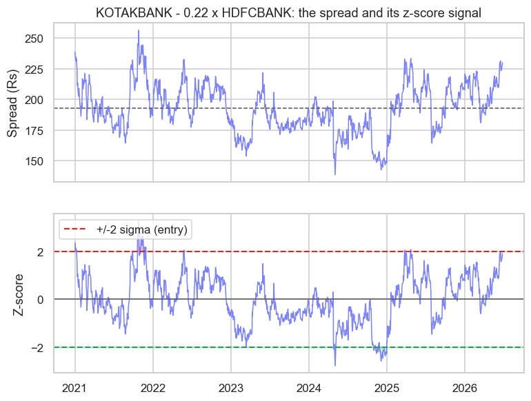
The top panel is the Kotak-minus-HDFC spread oscillating around its mean near Rs 193; the bottom panel is the same series as a z-score with the trading bands drawn in. The rule is mechanical. When the z-score climbs above +2 (red), the spread is unusually stretched, so you short it - sell the rich leg, buy the cheap one - and wait for the snap back. When it falls below -2 (green), you buy the spread. You exit as it crosses zero, back at fair value. Over this window the spread breached the two-sigma bands on 73 separate days, each a candidate trade, and not one required a view on where the market was heading. The latest reading is +1.92, a whisker below the short band - close to a live setup as I write.

Selecting Indian pairs

Good pairs come from a shared economic driver, not a data-mining sweep. Hunt where two names are pulled by the same force: two private banks, two public-sector oil marketers, two cement makers, a heavyweight stock against its sector index, or two arms of the same group. Then demand both an economic story and a passing test. We screened three logical pairs and only one survived - that hit rate is normal, and it is healthy. A pair that passes the test with no economic tether is a coincidence waiting to revert to chaos, while a pair with a strong story but a failing test is simply not ready to trade. Before committing, re-test on sub-samples to check the bond held throughout, and estimate the half-life (Chapter 44) to decide whether the holding period suits you.

When the spring snaps

Everything above rests on a statistical relationship, and statistics are not laws of nature. A merger, a regulatory shift, a strategic divergence where one bank reinvents itself, an index reconstitution, or a large corporate action can cut the tether for good. The spread that "always reverts" then walks away and never returns, and the mean-reversion trade quietly mutates into averaging down on a permanent loss. The asymmetry is brutal: your profit is capped at the spread returning to its mean, but a broken spread's loss is open-ended.

The defences are concrete. Set a hard stop - if the z-score blows past a wide band such as 3.5 or 4, exit rather than add. Re-test the cointegration on a rolling basis and drop dead pairs. Cost both legs honestly, including the borrow or securities-lending fee on the short side (Chapter 28), because a pairs trade pays two spreads, not one. And keep watching the half-life: a reverting spread that suddenly takes far longer to come home is often a relationship in the act of breaking.

Pairs trading is the cleanest expression of market-neutral thinking - profit from a relationship, not a direction. We will scale it into a full statistical-arbitrage book in Module G (Chapter 63). But first, Chapter 46 tackles the question lurking behind every snapped spring: how do you detect the regime shifts and structural breaks that end a working strategy, ideally before they end your capital?