HFT Strategy Families: Making, Arb and Event

Last chapter proved you cannot win the speed race - a colocated engine reacts in microseconds while your round trip takes hundreds of milliseconds. So a fair question is: what exactly are those microsecond machines doing with all that speed? It turns out the answer is not exotic. HFT runs three classic trading jobs you already half understand - making markets, arbitraging prices, and reacting to events - just executed faster than perception and fully automated. Understanding these families tells you which corners of the market are owned by speed (leave them) and which reward research and patience (yours to take). This chapter is the map; later chapters drill into the two families that matter most for a thinking quant.

Three families, one automated book

Almost every HFT strategy is a variation on three edges. Each earns money a different way and dies a different way, and a real HFT firm usually runs all three at once across thousands of instruments.

Family one: passive market making

A market maker posts a resting buy order (a bid) and a resting sell order (an ask) on the same instrument, slightly apart. When a buyer crosses the ask and a seller crosses the bid, the maker has bought low and sold high, pocketing the spread without taking a view on direction. Do this on a few thousand symbols, a few thousand times a second, and tiny per-trade margins add up.

The edge sounds free. It is not. The maker's nightmare is adverse selection: the people who hit your quote often know something you don't. If informed flow keeps lifting your ask just before the price jumps, you are systematically selling to the better-informed and your "spread profit" turns into a loss. The second enemy is inventory risk - every fill leaves you holding a position you did not choose, and if the market trends against that accidental inventory you bleed. A market maker's whole craft is managing these two: skewing quotes to lean against inventory, widening when toxicity rises, and pulling quotes entirely in a fast market. We give this its own full treatment, including the Avellaneda-Stoikov quoting model, in the market-making and inventory-risk chapter (ch38).

Family two: arbitrage at speed

Arbitrage is the purest HFT edge: the same economic value is momentarily priced two different ways, and you take both sides to lock the difference. Two flavours dominate.

Latency arbitrage exploits the same instrument trading on two venues. NIFTY constituents trade on more than one exchange; an index future moves a beat before its basket; an ETF drifts from its underlying. When one quote updates and the other has not yet caught up, there is a risk-free gap for whoever reaches both order books first. The word first is doing all the work - this is a pure speed game, decided by colocation and wire length, and it is utterly closed to a retail quant (see ch31 on why physics, not code, sets the limit).

Statistical arbitrage at speed is the one a thinking quant can actually study. Instead of an exact price equality, you trade a statistical relationship: two related names that usually move together, an index against its components, a stock against its future. You build a spread - one leg minus a hedge ratio times the other - and trade it when it stretches unusually far from its own average, betting it snaps back. HFT runs this on micro-dislocations that vanish in milliseconds; you would run the identical logic on minutes or days. The full market-neutral version, with cointegration and portfolio construction, is chapter 62; the pairs-trading mechanics and the Engle-Granger test are chapter 45. Here, let us just see the signal on real bank data.

# A micro stat-arb signal: spread z-score on two related Nifty bank names at 1m.
import os

import numpy as np
import pandas as pd
from openalgo import api

client = api(
    api_key=os.getenv("OPENALGO_API_KEY", "your_api_key_here"),
    host=os.getenv("OPENALGO_HOST", "http://127.0.0.1:5000"),
)

A, B = "HDFCBANK", "ICICIBANK"
start, end = "2026-06-16", "2026-06-27"
ca = client.history(symbol=A, exchange="NSE", interval="1m", start_date=start, end_date=end)["close"]
cb = client.history(symbol=B, exchange="NSE", interval="1m", start_date=start, end_date=end)["close"]

px = pd.concat([ca, cb], axis=1, keys=[A, B]).dropna()
ret_corr = px[A].pct_change().corr(px[B].pct_change())

# hedge ratio from a simple OLS fit, then the spread and its rolling z-score
beta = np.polyfit(px[B], px[A], 1)[0]
spread = px[A] - beta * px[B]
win = 60
z = (spread - spread.rolling(win).mean()) / spread.rolling(win).std()
px = px.assign(spread=spread, z=z).dropna()

extreme = px[px["z"].abs() >= 2.0].copy()
extreme["signal"] = np.where(extreme["z"] >= 2, "short spread (sell A / buy B)",
                             "long spread (buy A / sell B)")

print(f"Pair {A} vs {B} on 1m bars : {len(px)} usable bars, return corr {ret_corr:.2f}")
print(f"Hedge ratio A = {beta:.3f} * B, z window {win} bars, current z = {px['z'].iloc[-1]:+.2f}")
print(f"Extreme bars |z| >= 2 : {len(extreme)}  ({100*len(extreme)/len(px):.1f}% of the session)")
print("\nLast 5 entry candidates:")
print(extreme[["z", "signal"]].tail(5).round(2).to_string())

Pair HDFCBANK vs ICICIBANK on 1m bars : 2941 usable bars, return corr 0.25
Hedge ratio A = 0.170 * B, z window 60 bars, current z = -1.09
Extreme bars |z| >= 2 : 430  (14.6% of the session)

Last 5 entry candidates:
                              z                        signal
timestamp                                                    
2026-06-25 15:05:00+05:30 -2.58  long spread (buy A / sell B)
2026-06-25 15:06:00+05:30 -2.62  long spread (buy A / sell B)
2026-06-25 15:07:00+05:30 -2.35  long spread (buy A / sell B)
2026-06-25 15:08:00+05:30 -2.10  long spread (buy A / sell B)
2026-06-25 15:11:00+05:30 -2.12  long spread (buy A / sell B)

The script fits a hedge ratio between HDFCBANK and ICICIBANK (about 0.170 over this window), forms the spread, and standardises it into a rolling z-score - how many standard deviations the spread sits from its own 60-bar mean. A z above +2 says the spread is unusually rich (sell A, buy B); below -2 says it is unusually cheap (buy A, sell B). On the last 2,941 one-minute bars the current z was -1.09, and the last five entry candidates were all "long spread" as the gap stretched into the close.

But read the honest number underneath: 430 of those bars, fully 14.6 percent, sat beyond two sigma, far more than the roughly 5 percent a clean mean-reverting series would give. And the return correlation between the two names was only 0.25. That is the trap in one statistic - this pair is not cleanly cointegrated, the spread drifts and trends, so a naive z-score fires constantly and a real book would be run over. The signal is the easy part; deciding the relationship is stable enough to bet on is the hard part.

Now the same data as a picture - the two normalised price paths and the spread's z-score with its entry bands:

Copy

# Chart the two normalised prices and their spread z-score with entry bands.
import os
from pathlib import Path

import matplotlib

matplotlib.use("Agg")
import matplotlib.pyplot as plt
import numpy as np
import pandas as pd
import seaborn as sns
from openalgo import api

client = api(
    api_key=os.getenv("OPENALGO_API_KEY", "your_api_key_here"),
    host=os.getenv("OPENALGO_HOST", "http://127.0.0.1:5000"),
)

A, B = "HDFCBANK", "ICICIBANK"
start, end = "2026-06-16", "2026-06-27"
ca = client.history(symbol=A, exchange="NSE", interval="1m", start_date=start, end_date=end)["close"]
cb = client.history(symbol=B, exchange="NSE", interval="1m", start_date=start, end_date=end)["close"]

px = pd.concat([ca, cb], axis=1, keys=[A, B]).dropna().reset_index(drop=True)
norm = px / px.iloc[0] * 100.0          # both start at 100 so the co-movement is visible

beta = np.polyfit(px[B], px[A], 1)[0]
spread = px[A] - beta * px[B]
win = 60
z = (spread - spread.rolling(win).mean()) / spread.rolling(win).std()

sns.set_theme(style="whitegrid")
fig, (ax1, ax2) = plt.subplots(2, 1, figsize=(9, 6.5), sharex=True)

ax1.plot(norm[A], color="#7c83ff", lw=1.2, label=A)
ax1.plot(norm[B], color="#16a34a", lw=1.2, label=B)
ax1.set_title("Two bank names, normalised to 100 - they wander together")
ax1.set_ylabel("Normalised price")
ax1.legend(loc="upper left")

ax2.plot(z, color="#334155", lw=1.0)
for band, style in [(0, "-"), (1, ":"), (-1, ":"), (2, "--"), (-2, "--")]:
    ax2.axhline(band, color="#dc2626" if abs(band) == 2 else "#9a9a9a",
                ls=style, lw=1.0 if abs(band) == 2 else 0.8)
ax2.fill_between(z.index, 2, z, where=(z >= 2), color="#dc2626", alpha=0.25)
ax2.fill_between(z.index, -2, z, where=(z <= -2), color="#dc2626", alpha=0.25)
ax2.set_title("Spread z-score - red bands at +/-2 are the entry triggers")
ax2.set_ylabel("z-score")
ax2.set_xlabel("1-minute bars")

out = Path(__file__).with_suffix(".png")
plt.savefig(out, dpi=110, bbox_inches="tight")
n_hits = int((z.abs() >= 2).sum())
print(f"Plotted {len(px)} 1m bars; hedge ratio {beta:.3f}; {n_hits} bars beyond +/-2 sigma. Saved {out.name}")

Live output

Plotted 3000 1m bars; hedge ratio 0.170; 430 bars beyond +/-2 sigma. Saved 02_spread_zscore_chart.png

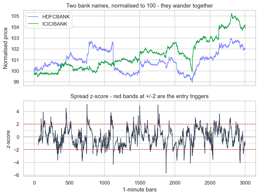
The top panel shows both names rebased to 100 so their co-movement is visible; the lower panel is the z-score, with red bands at plus and minus two standard deviations shading every breach. You can see at a glance how often the spread pokes through the bands and, crucially, how it sometimes keeps going instead of snapping back - the visual signature of a drifting relationship.

Family three: event reaction and liquidity detection

The third family trades information and the order book itself rather than a steady spread or a price gap.

Event reaction means parsing a scheduled or breaking event - an RBI rate decision, a results announcement, an index-inclusion notice, even a machine-readable economic print - and trading the move in the milliseconds before slower participants digest it. The edge is being first to a genuine signal; the risk is acting on a false or misread one and getting whipsawed when the crowd fades the initial spike.

Liquidity detection is more subtle and more controversial. Fast players probe the book with small orders to infer where large hidden interest sits - sniffing out an iceberg order or a big institutional buyer - then trade ahead of the size they have detected. The honest version is simply reading supply and demand; the abusive versions (spoofing, layering, quote stuffing) are market manipulation, watched closely by exchange surveillance and penalised through the order-to-trade ratio regime we cover in chapter 35.

The HFT book's risk

What unites all three families is not the edge but the risk discipline. An HFT book makes thousands of tiny bets, so its profit per trade is microscopic and a single fat loss can erase a whole day. That forces a particular shape of risk management: hard inventory caps per instrument, automatic quote-pulling when toxicity or volatility spikes, kill switches that flatten everything in a heartbeat, and obsessive control of the order-to-trade ratio so the firm is not fined or flagged for over-quoting. The strategies look like speed; the survival comes from limits. We build exactly these controls - pre-trade gates and kill switches - in chapter 40.

These three families recur throughout the rest of the course, slowed down to horizons you can compete on. Next we turn to the metric that polices all of them on the exchange's side - the order-to-trade ratio - and the line between legitimate quoting and manipulation.