Multiple Testing and False Discovery

The previous chapter showed you the trap: search enough zero-edge ideas and luck hands you a gorgeous winner. That was the diagnosis. This chapter is the treatment. A quant who knows the multiple-testing trap exists but has no formal way to price it will still get fooled, because intuition badly underestimates how fast false positives accumulate. So we make it exact. We will put a number on "how surprised should I be, given that I tried two hundred things," and we will build the small toolbox - family-wise error control, the false discovery rate, and the deflated Sharpe - that separates a result worth funding from a coincidence wearing a costume.

When one test becomes a family

Recall the bargain of a p-value: a 5% significance level means that if there is no edge, a result this strong appears at most 5% of the time. Test one strategy and you accept a 1-in-20 chance of being fooled. Reasonable. But the moment you test a family of hypotheses - many strategies, many parameters, many symbols - the relevant question is no longer "will this one test mislead me" but "will any test in the whole batch mislead me." That batch-level risk is the family-wise error rate (FWER): the probability of at least one false positive across everything you tried.

The arithmetic is brutal. If each of N independent zero-edge tests has a 5% chance of a false positive, the chance that none fires is 0.95 to the power N, so the FWER is 1 minus that. For N = 20 it is already 64%. For N = 200 it is 0.99997 - a false discovery is not a risk, it is a near-certainty. You will find something. You are guaranteed to find something. The only question is whether you mistake it for skill.

Let us make it concrete on real Nifty. We generate 200 signals that are pure noise - random long/short rules with no edge by construction - run a proper one-sample t-test on each strategy's daily P&L, and count how many clear the usual bar.

# Test 200 zero-edge signals on real Nifty, count false discoveries at p<0.05, then correct.
import os
from datetime import datetime

import numpy as np
from openalgo import api
from scipy import stats
from statsmodels.stats.multitest import multipletests

client = api(
    api_key=os.getenv("OPENALGO_API_KEY", "your_api_key_here"),
    host=os.getenv("OPENALGO_HOST", "http://127.0.0.1:5000"),
)

end = datetime.now().strftime("%Y-%m-%d")
r = client.history(symbol="NIFTY", exchange="NSE_INDEX", interval="D",
                   start_date="2018-01-01", end_date=end)["close"].pct_change().dropna().values

rng = np.random.default_rng(7)
N, days = 200, len(r)

# Each "signal" is a random long/short rule with NO real edge. Test its daily P&L.
pvals = np.empty(N)
for i in range(N):
    signal = rng.choice([1, -1], size=days)        # pure noise, expected edge = 0
    pnl = signal * r
    pvals[i] = stats.ttest_1samp(pnl, 0.0).pvalue   # H0: mean daily return = 0

naive = (pvals < 0.05).sum()
bonf = multipletests(pvals, alpha=0.05, method="bonferroni")[0].sum()
holm = multipletests(pvals, alpha=0.05, method="holm")[0].sum()
bh = multipletests(pvals, alpha=0.05, method="fdr_bh")[0].sum()

print(f"Tested {N} ZERO-edge signals on {days} days of Nifty (2018 to date).")
print(f"Naive p<0.05            : {naive:3d} 'discoveries'  (expected by luck ~{int(0.05*N)})")
print(f"Bonferroni (FWER 5%)    : {bonf:3d} survive   threshold p<{0.05/N:.5f}")
print(f"Holm step-down (FWER 5%): {holm:3d} survive")
print(f"Benjamini-Hochberg FDR  : {bh:3d} survive")
print(f"\n{naive} fake edges passed the naive test; corrections killed all but {max(bonf, holm, bh)} of them.")

Tested 200 ZERO-edge signals on 2100 days of Nifty (2018 to date).
Naive p<0.05            :  11 'discoveries'  (expected by luck ~10)
Bonferroni (FWER 5%)    :   0 survive   threshold p<0.00025
Holm step-down (FWER 5%):   0 survive
Benjamini-Hochberg FDR  :   0 survive

11 fake edges passed the naive test; corrections killed all but 0 of them.

Eleven of the two hundred zero-edge signals produced a t-statistic significant at p < 0.05, almost exactly the ten that pure luck predicts (5% of 200). Every one is a false discovery. Reported in isolation, any of those eleven would look like a real edge. The fix is not to test fewer ideas - it is to raise the bar in proportion to how hard you searched.

Bonferroni and Holm: bounding the worst case

The bluntest fix is the Bonferroni correction: to hold the family-wise error at 5% across N tests, demand that each individual test clear 0.05 / N instead of 0.05. For our 200 signals that threshold becomes p < 0.00025, and as the example shows, zero of the eleven naive winners survive it. Bonferroni traded eleven confident mistakes for an honest "nothing here," which is exactly the right answer when the data is noise.

Bonferroni is correct but conservative. By guarding against the worst case - tests that are perfectly independent and all null - it throws away real discoveries when you have many tests, because the threshold gets punishingly small. The Holm step-down procedure recovers some of that power while keeping the identical FWER guarantee. You sort the p-values from smallest to largest and compare the smallest to 0.05 / N, the next to 0.05 / (N-1), the next to 0.05 / (N-2), and so on, stopping the first time a test fails. It is uniformly more powerful than plain Bonferroni and there is no reason to prefer Bonferroni once you know it. On our noise data both agree - nothing survives - because there was never anything to find.

The false discovery rate: a kinder bar

Family-wise control asks for something very strict - zero false positives in the whole family - and that is the right standard when a single mistake is expensive (going live with a fake strategy and real capital). But when you are screening thousands of candidates in a research pipeline and simply want a shortlist worth deeper study, demanding zero false positives leaves you with almost nothing. Here the better idea is to control not the chance of any error but the expected proportion of errors among the things you flag. That proportion is the false discovery rate (FDR).

The Benjamini-Hochberg procedure implements it. Sort the N p-values ascending, and find the largest rank k whose p-value is below k/N times your chosen rate q (say q = 0.05). Reject everything up to that rank. The promise is softer but honest: of the discoveries you keep, no more than about 5% are expected to be false. On our pure-noise example BH also returns nothing, which is correct - there are no true effects to discover, so even a lenient rule finds none.

Data snooping and the deflated Sharpe

The corrections above assume you counted your tests. The deadliest version of this bias is the one you do not count: data snooping, where the search is informal and invisible. You try an indicator, eyeball the equity curve, tweak the lookback, swap the symbol, adjust the stop - and report only the version that looked best. There is no list of p-values to correct because you never wrote the tries down. But every glance at the data was a test, and the reported result is a maximum over a search you have hidden even from yourself.

The clean way to see selection inflation is to ask what the best result out of N pure-luck tries looks like. The maximum of N draws from a zero-mean distribution drifts steadily rightward as N grows - not because anything is real, but because you are sampling the extreme of a wider and wider net. Statisticians know this curve exactly: the expected maximum of N standard draws grows roughly like the square root of twice the log of N. Scale that by the standard error of a Sharpe estimate over your sample and you get the hurdle a backtest must clear merely to be unremarkable.

Copy

# Best-of-N backtest Sharpe inflates with N - and tracks the expected max under the null.
import os
from datetime import datetime
from pathlib import Path

import matplotlib

matplotlib.use("Agg")
import matplotlib.pyplot as plt
import numpy as np
import seaborn as sns
from openalgo import api
from scipy.stats import norm

client = api(
    api_key=os.getenv("OPENALGO_API_KEY", "your_api_key_here"),
    host=os.getenv("OPENALGO_HOST", "http://127.0.0.1:5000"),
)

end = datetime.now().strftime("%Y-%m-%d")
r = client.history(symbol="NIFTY", exchange="NSE_INDEX", interval="D",
                   start_date="2018-01-01", end_date=end)["close"].pct_change().dropna().values

rng = np.random.default_rng(11)
days, M, reps = len(r), 2000, 40
ann = np.sqrt(252.0)

# Empirical best-of-k: average the running max of k random (zero-edge) Sharpes over many reps.
best_curves = np.empty((reps, M))
for j in range(reps):
    sig = rng.integers(0, 2, size=(M, days)) * 2 - 1     # M random +/-1 strategies
    pnl = sig * r
    sharpe = pnl.mean(axis=1) / pnl.std(axis=1) * ann
    best_curves[j] = np.maximum.accumulate(sharpe)
best_of_n = best_curves.mean(axis=0)

# Theory: expected max of N iid standard normals, scaled by the null Sharpe std-error.
sr_se = np.sqrt(252.0 / days)
emc = 0.5772156649
n = np.arange(1, M + 1)
exp_max = np.where(n < 2, 0.0,
                   (1 - emc) * norm.ppf(1 - 1.0 / np.maximum(n, 2))
                   + emc * norm.ppf(1 - 1.0 / (np.maximum(n, 2) * np.e)))
hurdle = sr_se * exp_max

sns.set_theme(style="whitegrid")
fig, ax = plt.subplots(figsize=(8, 4.5))
ax.plot(n, best_of_n, color="#7c83ff", lw=2, label="best-of-N random Sharpe (simulated)")
ax.plot(n, hurdle, color="#dc2626", lw=1.8, ls="--", label="expected max under null (selection hurdle)")
ax.set_xscale("log")
ax.set_xlabel("N strategies searched")
ax.set_ylabel("Annualised Sharpe of the winner")
ax.set_title("Selection inflation: the best of N zero-edge strategies")
ax.legend(loc="upper left")

out = Path(__file__).with_suffix(".png")
plt.savefig(out, dpi=110, bbox_inches="tight")
print(f"Best-of-{M} random Sharpe averaged {best_of_n[-1]:.2f}; the null predicts a max of {hurdle[-1]:.2f}. "
      f"All luck, no edge. Saved {out.name}")

Live output

Best-of-2000 random Sharpe averaged 1.16; the null predicts a max of 1.19. All luck, no edge. Saved 02_selection_inflation.png

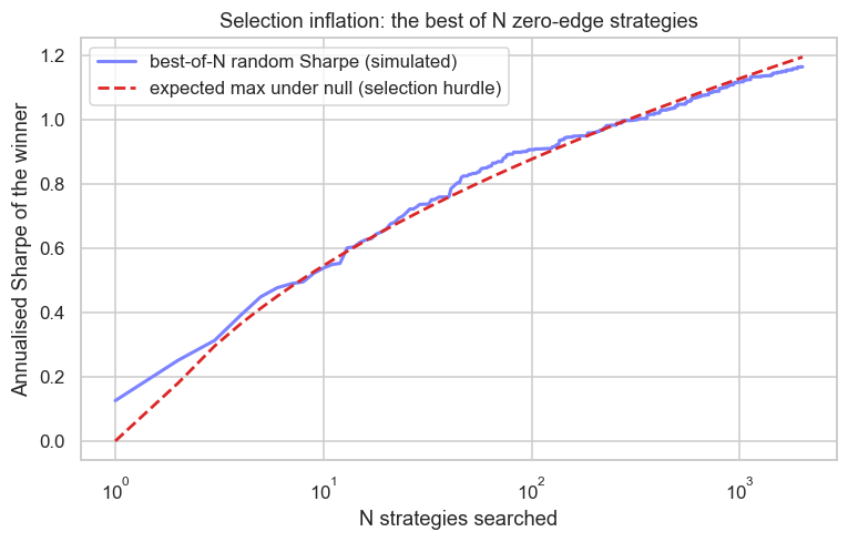
The simulated best-of-N curve and the theoretical null hurdle sit almost on top of each other: search 2000 zero-edge strategies on Nifty and the winner averages a Sharpe of 1.16, while the null alone predicts an expected maximum of 1.19. A Sharpe near 1.2, which most traders would happily fund, is exactly what you should expect from luck after a search that size. The number that should impress you is not the winner's Sharpe but how far it clears the hurdle for the N you searched.

This is precisely what the deflated Sharpe ratio of Bailey and Lopez de Prado formalises. It takes your observed Sharpe and discounts it for three things: the number of trials you ran, the variance of the Sharpes across those trials, and the non-normality (skew and fat tails) of the returns. The output is the probability that your edge is real after honestly accounting for the search. A raw Sharpe of 1.2 from one clean test and the same 1.2 selected as the best of two thousand are not the same evidence, and the deflated Sharpe is the tool that prices the difference.

A protocol you can actually follow

You do not need to memorise every procedure. You need a habit:

• Count and log every test, including the informal eyeballing. N is the search size, not the number of scripts you ran.
• Pick the bar to the job. Going live means FWER (Holm over Bonferroni, same guarantee, more power). Screening a universe means FDR (Benjamini-Hochberg).
• Deflate the headline. Judge a Sharpe against the expected maximum for your N, or compute the deflated Sharpe outright. If the winner barely clears the luck hurdle, it is luck.
• Spend your significance budget. Reserve a truly untouched slice of data and test the survivor on it exactly once. That single honest test is worth more than any correction applied to data you have already mined.

We have now built the immune system: in the previous chapter, the intuition that search manufactures luck, and in this one, the exact tools to price and defend against it. Next we turn from "is this edge real" to a deeper question about the game itself - whether prices are predictable at all. We meet stationarity, the random walk, and what the efficient-market hypothesis genuinely claims about the market we are trying to beat.