Realized and Intraday Volatility

A daily close hides almost everything. Between yesterday's 15:30 print and today's, NIFTY may have drifted sleepily or whipsawed through three reversals, gapped on an overnight cue, and stampeded into the close - and a single close-to-close return collapses all of it into one number. The previous chapter forecast volatility from those daily returns with GARCH. This chapter does something different and more precise: it measures volatility directly from the high-frequency record of the day itself. When you have 5-minute bars instead of one close, you stop estimating variance from a handful of noisy points and start summing it up move by move. That idea - realized volatility - is the bridge between daily time-series models and the microstructure world of Module C, and it quietly underpins how modern desks mark risk.

Realized variance: volatility you add up, not estimate

The classical estimate of variance is the sample variance of close-to-close returns: take a month of daily moves, square the deviations, average. With twenty or thirty observations it is a blunt instrument, swinging around with every outlier. Realized variance takes the opposite approach. Slice the trading day into many short intervals, compute the return over each, and sum the squared returns. Under a sensible model of prices, that sum converges to the day's true variance as the intervals get finer. One day of 5-minute bars gives roughly 74 intraday returns - far more information than the single number a daily close provides.

The realized volatility for a day is the square root of that sum; annualise by scaling with the square root of 252 trading days. Let us compute it for NIFTY and stand it next to the naive close-to-close estimate over the same window.

# Realized volatility from 5m intraday bars vs a plain close-to-close estimate, for NIFTY.
import os
from datetime import datetime

import numpy as np
from openalgo import api

client = api(
    api_key=os.getenv("OPENALGO_API_KEY", "your_api_key_here"),
    host=os.getenv("OPENALGO_HOST", "http://127.0.0.1:5000"),
)

end = datetime.now().strftime("%Y-%m-%d")
df = client.history(symbol="NIFTY", exchange="NSE_INDEX", interval="5m",
                    start_date="2026-03-01", end_date=end)

px = df["close"]
day = px.index.normalize()                                  # session date for each bar

# Intraday 5m log returns WITHIN each session (groupby drops the overnight gap)
logret = np.log(px).groupby(day).diff().dropna()
rv_day = (logret ** 2).groupby(logret.index.normalize()).sum()   # realized variance per day

ann_rv = np.sqrt(rv_day.mean() * 252) * 100                 # annualised realized vol (intraday, open-to-close)

# Plain close-to-close: one daily return per session, then its sample volatility
daily_close = px.groupby(day).last()
cc_ret = np.log(daily_close).diff().dropna()
ann_cc = cc_ret.std() * np.sqrt(252) * 100                  # annualised close-to-close vol (includes overnight)

n_days = int(rv_day.shape[0])
bars = int(logret.groupby(logret.index.normalize()).size().median())

print(f"NIFTY realized vs close-to-close volatility  ({n_days} sessions, ~{bars} five-min returns/day)")
print(f"  Realized vol (5m intraday, open-to-close) : {ann_rv:5.1f}%  annualised")
print(f"  Close-to-close vol (daily)                : {ann_cc:5.1f}%  annualised")
print(f"  Gap (overnight + sampling difference)     : {ann_cc - ann_rv:+5.1f} pts")
print(f"SUMMARY: 5m realized vol {ann_rv:.1f}% vs close-to-close {ann_cc:.1f}% annualised "
      f"({n_days} sessions); the {ann_cc - ann_rv:+.1f} pt gap is risk the intraday measure misses.")

NIFTY realized vs close-to-close volatility  (77 sessions, ~74 five-min returns/day)
  Realized vol (5m intraday, open-to-close) :  11.2%  annualised
  Close-to-close vol (daily)                :  18.7%  annualised
  Gap (overnight + sampling difference)     :  +7.5 pts
SUMMARY: 5m realized vol 11.2% vs close-to-close 18.7% annualised (77 sessions); the +7.5 pt gap is risk the intraday measure misses.

Over 77 recent sessions the intraday 5-minute realized vol prints at 11.2% annualised, while the close-to-close estimate prints at 18.7% - a gap of 7.5 points. That gap is not an error. It is the single most important lesson in this chapter, and we return to it below: the intraday measure deliberately ignores the overnight move, and overnight risk is real.

How fast should you sample? Microstructure noise

If finer is better, why not use 1-second data and sum millions of squared returns? Because at high frequency you stop measuring the price and start measuring the plumbing. Every print bounces between the bid and the ask, ticks sit on a discrete grid, and quotes flicker. These microstructure effects add a spurious, mean-reverting wiggle to the return series. Squaring and summing that wiggle inflates realized variance with pure noise. Sample too slowly, on the other hand, and you throw away genuine intraday information and get a high-variance, jumpy estimate.

This is a bias-variance trade-off with a famous diagnostic: the volatility signature plot, where you compute realized variance at many sampling frequencies and watch the estimate blow up as the interval shrinks toward the tick. The practitioner's compromise for liquid Indian index and large-cap names has long been the 5-minute bar - slow enough that bid-ask bounce averages out, fast enough to capture the day's structure. That is exactly why the example above used 5-minute data rather than 1-minute or tick.

The intraday U-shape

Volatility is not spread evenly across the day. Trading concentrates at the boundaries: the opening auction releases the entire overnight order imbalance at once, and the close draws in funds marking to the settlement price, expiry hedgers, and anyone who must be flat by 15:30. The quiet middle - roughly the lunch hours - sees the thinnest flow and the smallest moves. Plot average absolute return against the minute of the day and this U-shape (more precisely a reverse-J: a tall open, a low trough, a firm rise into the close) appears with remarkable stability.

Let us measure it on a real large-cap rather than draw it from memory.

Copy

# The intraday volatility U-shape: average absolute 1m return by minute-of-day for RELIANCE.
import os
from datetime import datetime
from pathlib import Path

import numpy as np
import matplotlib

matplotlib.use("Agg")
import matplotlib.pyplot as plt
import seaborn as sns
from openalgo import api

client = api(
    api_key=os.getenv("OPENALGO_API_KEY", "your_api_key_here"),
    host=os.getenv("OPENALGO_HOST", "http://127.0.0.1:5000"),
)

end = datetime.now().strftime("%Y-%m-%d")
df = client.history(symbol="RELIANCE", exchange="NSE", interval="1m",
                    start_date="2026-03-01", end_date=end)

px = df["close"]
# 1m log returns within each session (overnight gap dropped), in basis points
ret = (np.log(px).groupby(px.index.normalize()).diff().dropna().abs()) * 1e4
tod = ret.index.strftime("%H:%M")
profile = ret.groupby(tod).mean()                 # average |return| by minute-of-day
profile = profile.sort_index()

x = np.arange(len(profile))
sns.set_theme(style="whitegrid")
fig, ax = plt.subplots(figsize=(8, 4.5))
ax.plot(x, profile.values, color="#7c83ff", lw=1.6)
ax.fill_between(x, profile.values, color="#7c83ff", alpha=0.12)
ticks = [t for t in ["09:15", "10:30", "12:00", "13:30", "15:00", "15:29"] if t in profile.index]
ax.set_xticks([profile.index.get_loc(t) for t in ticks])
ax.set_xticklabels(ticks)
ax.set_title("RELIANCE - average absolute 1m return by minute of day (the intraday U-shape)")
ax.set_ylabel("Mean |return| (basis points)")
ax.set_xlabel("Time of day (IST)")

out = Path(__file__).with_suffix(".png")
plt.savefig(out, dpi=110, bbox_inches="tight")

open_v = profile.iloc[:15].mean()                 # first ~15 min
mid_v = profile.loc["12:00":"13:00"].mean()       # lunch lull
close_v = profile.iloc[-15:].mean()               # last ~15 min
print(f"RELIANCE intraday vol U-shape: open {open_v:.1f} bps, midday {mid_v:.1f} bps, close {close_v:.1f} bps "
      f"per minute -> open is {open_v / mid_v:.1f}x the midday lull. Saved {out.name}")

Live output

RELIANCE intraday vol U-shape: open 9.3 bps, midday 3.7 bps, close 4.5 bps per minute -> open is 2.5x the midday lull. Saved 02_intraday_ushape.png

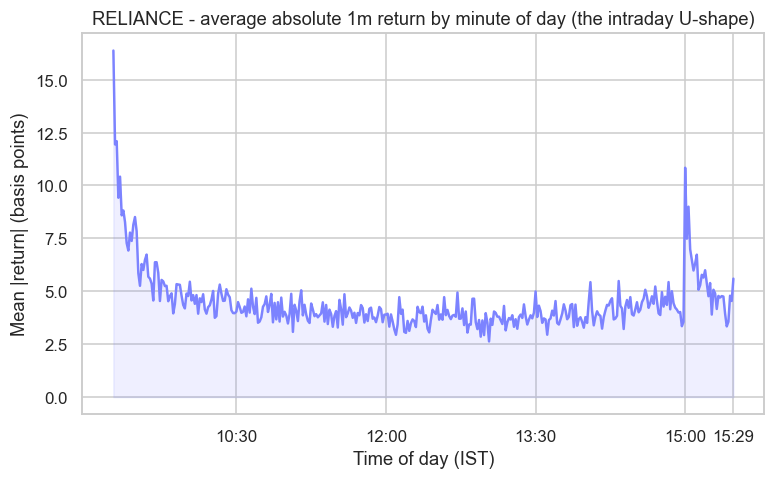
For RELIANCE the first minutes average about 9.3 basis points of absolute move per minute, the midday hours sink to roughly 3.7 basis points, and the final stretch firms back to 4.5 basis points. The open carries about 2.5 times the per-minute volatility of the quiet midday window. This shape is not a curiosity, it is a design input. An execution algorithm that slices an order evenly across the clock will trade most of it through the noisy, expensive boundaries; a VWAP or arrival-price schedule deliberately leans into the cheaper middle and treats the open and close with care.

Overnight versus intraday risk

Now back to that 7.5-point gap. The realized measure summed only intraday 5-minute returns, so by construction it knows nothing about what happened between 15:30 and the next 09:15. The close-to-close estimate, by contrast, spans that gap - it carries the overnight jump on every cue that lands while the cash market is shut: global moves, results announced after hours, policy decisions, currency swings. In this window that overnight component was large enough that close-to-close vol nearly doubled the intraday figure.

The practical consequences are sharp. A position held flat at the close still carries full overnight risk, and you cannot trade through it - there is no continuous Indian equity session at 02:00. A complete realized-variance estimator therefore adds the squared overnight return as one extra term to the intraday sum, restoring the missing risk. For a quant deciding whether to hold or square off by 15:30, separating the two is essential: intraday-only strategies face the U-shaped, hedgeable risk above, while anything carried overnight inherits a fat, un-hedgeable gap.

Realized versus implied

Realized volatility is backward-looking: it is the verdict on how turbulent the market actually was, measured from the tape. India VIX and option prices give you the other half - implied volatility, the market's forward-looking, risk-priced expectation of how turbulent it will be. These two are not the same number, and their difference is itself a tradeable quantity. Implied vol typically sits above subsequent realized vol, and that persistent wedge is the variance risk premium - the compensation option sellers earn for bearing the risk of a volatility spike. Measuring realized vol cleanly, as this chapter does, is the prerequisite for ever quantifying that premium honestly; we return to it with India VIX in Module F.

Recap

• Realized variance sums squared high-frequency returns; with ~74 five-minute bars a day it measures the day's volatility far more precisely than a few daily closes.
• For NIFTY the 5-minute realized vol printed at 11.2% against a close-to-close estimate of 18.7% - the 7.5-point gap is the overnight move the intraday measure omits.
• Microstructure noise (bid-ask bounce, tick discreteness) inflates realized variance if you sample too fast; the 5-minute bar is the standard compromise, read off a volatility signature plot.
• The intraday U-shape is real and stable: RELIANCE moved about 9.3 bps/min at the open versus 3.7 bps/min midday, roughly 2.5 times as volatile at the boundaries.
• Overnight versus intraday risk are different animals, and realized versus implied volatility is the backward-versus-forward distinction at the heart of the variance risk premium.

You can now measure volatility precisely from inside the day, separate when and where it lives, and tell the realized past from the implied future. The next step in the module leaves single-series volatility behind and turns to the relationship between two prices - the mean-reverting spread that powers cointegration and pairs trading.