Mean Reversion and Ornstein-Uhlenbeck

Most of what a forecaster does is an uphill fight. A stock price is close to a random walk, so guessing tomorrow's level from today's is mostly a fool's errand - the price has no memory of where it has been. But a small and precious family of series behaves differently. They have a home. Push them away and a quiet force drags them back, again and again, with a strength you can actually measure and put a number on. This is mean reversion, and the cleanest mathematical model of it - a random walk kept on a leash to its own average - is the Ornstein-Uhlenbeck process. Learn to spot a genuinely reverting series, estimate how hard it is pulled home, and you hold the backbone of an entire class of trading strategies.

A price that remembers where it lives

A random walk wanders with no centre of gravity: each step is independent, and the best forecast of tomorrow is simply today. A mean-reverting series is the opposite. It has an equilibrium level, and the further it strays, the harder it is tugged back. Stretch it high and the next move leans down; push it low and the next move leans up.

Here is the catch that trips up every beginner: a raw stock price almost never reverts on its own. RELIANCE does not owe you a return to Rs 1,300 just because it sat there last month. What reverts are constructed quantities - deviations, ratios and spreads. A stock's gap from its own moving average, an index's distance from a long trend, the cash-futures basis (Chapter 50), a volatility measure, or the spread between two related names. These have an anchor by their very nature, and that anchor is what we model. Mean reversion is also the exact opposite of momentum: a momentum trader bets the recent move continues, a reversion trader bets it overshot and snaps back. The same series can do both on different horizons, which is why measuring the speed matters so much.

The Ornstein-Uhlenbeck process

The Ornstein-Uhlenbeck (OU) process writes that pull down in one short equation. If x is our series, its motion over a small step dt is

dx = kappa (theta - x) dt + sigma dW

Read it in three pieces. theta is home - the long-run mean the series is drawn toward. kappa (kappa) is the speed of mean reversion - how strongly it is pulled back per unit of time. sigma is the random buffeting (dW is the random shock) that keeps knocking it off course. The genius is in the drift term kappa (theta - x): when x sits above home the bracket is negative and the drift points down, when x is below home the drift points up, and the size of the pull grows with the distance. It is a spring, not a wall.

Discretise OU to daily steps and it becomes the humble AR(1) model you already half-know: x_t = c + phi * x_{t-1} + e_t, where phi = 1 - kappa. The whole story lives in phi. If phi is below 1 the series reverts, if phi equals 1 it is a pure random walk with no memory, and if phi exceeds 1 it explodes away. Estimating phi (or equivalently kappa) is therefore the entire job.

Estimating the speed and the half-life

Estimating kappa is a one-line regression. Rearrange the discrete OU as x_t - x_{t-1} = kappa*theta - kappa*x_{t-1} + noise: the daily change is a straight-line function of the lagged level. Regress the change on the level, and the slope is -kappa. A steep negative slope means a strong, fast pull; a slope near zero means a series that barely reverts, indistinguishable from a random walk.

We will run it on a series that ought to revert by construction: RELIANCE's log-distance from its own 20-day average. When the price runs ahead of its recent mean the gap is positive, when it lags the gap is negative, and the gap should oscillate around zero.

# Fit an Ornstein-Uhlenbeck / AR(1) model to one mean-reverting series and find its half-life.
import os
from datetime import datetime

import numpy as np
import statsmodels.api as sm
from openalgo import api
from statsmodels.tsa.stattools import adfuller

client = api(
    api_key=os.getenv("OPENALGO_API_KEY", "your_api_key_here"),
    host=os.getenv("OPENALGO_HOST", "http://127.0.0.1:5000"),
)

end = datetime.now().strftime("%Y-%m-%d")
px = client.history(symbol="RELIANCE", exchange="NSE", interval="D",
                    start_date="2021-01-01", end_date=end)["close"]

# One series that should mean-revert: the log-distance of price from its own 20-day average.
sma20 = px.rolling(20).mean()
x = np.log(px / sma20).dropna()                 # log-deviation, oscillates around ~0

# Does it TRULY revert? Augmented Dickey-Fuller: reject the unit root -> stationary -> reverts.
adf_p = adfuller(x, autolag="AIC")[1]

# OU discretised: dx = -kappa (x - theta) dt + noise. Regress the daily CHANGE on the LEVEL.
dx = x.diff().dropna()
lag = x.shift(1).loc[dx.index]
beta = sm.OLS(dx, sm.add_constant(lag)).fit().params
kappa = -beta.iloc[1]                            # speed of mean reversion, per day
theta = beta.iloc[0] / kappa                     # long-run mean it is pulled toward
halflife = np.log(2) / kappa                     # days to close half the gap

print("Ornstein-Uhlenbeck fit: RELIANCE log-deviation from its own 20-day average")
print(f"  ADF p-value     : {adf_p:.4f}  -> {'stationary, it truly reverts' if adf_p < 0.05 else 'cannot reject a random walk'}")
print(f"  reversion speed : kappa = {kappa:.3f} per day")
print(f"  long-run mean   : theta = {theta:+.4f}  (log-deviation, ~0 = price sits on its average)")
print(f"  half-life       : {halflife:.1f} days  (time to close half the gap back to the mean)")
print(f"SUMMARY: deviation reverts with kappa={kappa:.3f}/day, half-life {halflife:.1f} days, ADF p={adf_p:.3f}.")

Ornstein-Uhlenbeck fit: RELIANCE log-deviation from its own 20-day average
  ADF p-value     : 0.0000  -> stationary, it truly reverts
  reversion speed : kappa = 0.086 per day
  long-run mean   : theta = +0.0026  (log-deviation, ~0 = price sits on its average)
  half-life       : 8.0 days  (time to close half the gap back to the mean)
SUMMARY: deviation reverts with kappa=0.086/day, half-life 8.0 days, ADF p=0.000.

The fit is unambiguous. The reversion speed is kappa = 0.086 per day, and the long-run mean is theta = +0.0026 - essentially zero, meaning RELIANCE on average sits right on its own 20-day line, exactly as a deviation should. The Augmented Dickey-Fuller test (Chapter 14) returns a p-value below 0.0001, comfortably rejecting the random-walk null: this series is stationary, it genuinely reverts. But kappa = 0.086 is hard to feel. We need to translate the speed into time.

The translation is the half-life - the time it takes, on average, for a deviation to close half the distance back to its mean. For an OU process it is a clean formula:

half-life = ln(2) / kappa

With kappa = 0.086, the half-life is 0.693 / 0.086 = 8.0 days. So a stretched RELIANCE deviation gives back half its gap in about eight trading days, roughly a week and a half. That single number is the most useful output of the whole exercise, because it sets your natural holding period. A signal with an 8-day half-life is a swing trade, not a scalp and not a months-long position. If the half-life were one day, you would be trading almost intraday (Chapter 65); if it were sixty days, you would tie up capital for a quarter and absorb far more drift risk along the way.

Does it truly revert, or did you manufacture it?

Here is where honesty separates a quant from a curve-fitter. Our deviation passed the ADF test, but that is partly because we built it to. A distance from a moving average is a band-pass filter: subtracting a trailing mean mechanically removes the slow drift and leaves a wobble that looks stationary almost by definition. Passing ADF on such a constructed series is reassuring but not surprising. The harder questions are whether the reversion is strong enough to pay after costs, and whether it is stable - a series that reverts in calm markets can switch to trending in a regime change (Chapter 46), and your spring quietly becomes a slide.

Two disciplines keep you honest. First, beware look-ahead: the 20-day mean at any date must use only prices up to that date, which a trailing rolling mean does correctly, but it is an easy place to leak the future. Second, confirm reversion more than one way - the variance-ratio test is a useful companion to ADF, and re-estimating kappa on separate sub-samples shows whether the half-life is steady or wandering. A raw single price, tested directly, almost always fails these checks. That is the whole reason reverting deviations and spreads are precious.

Trading the reverting series

The trade is mechanical once the series is centred. Standardise the deviation into a z-score - how many standard deviations it sits from its mean - and fade the extremes: sell when it stretches high, buy when it stretches low, and exit as it returns to the mean. The half-life tells you how long the round trip should take, which doubles as a time-stop: if a position has not reverted in two or three half-lives, the relationship may have broken.

Copy

# One mean-reverting series: price vs its mean, and the deviation oscillating around zero.
import os
from datetime import datetime
from pathlib import Path

import matplotlib

matplotlib.use("Agg")
import matplotlib.pyplot as plt
import numpy as np
import seaborn as sns
import statsmodels.api as sm
from openalgo import api

client = api(
    api_key=os.getenv("OPENALGO_API_KEY", "your_api_key_here"),
    host=os.getenv("OPENALGO_HOST", "http://127.0.0.1:5000"),
)

end = datetime.now().strftime("%Y-%m-%d")
px = client.history(symbol="RELIANCE", exchange="NSE", interval="D",
                    start_date="2021-01-01", end_date=end)["close"]

sma20 = px.rolling(20).mean()
x = np.log(px / sma20).dropna()                 # log-deviation from the 20-day mean

# Half-life of reversion from the OU fit (regress the daily change on the level).
dx = x.diff().dropna()
lag = x.shift(1).loc[dx.index]
beta = sm.OLS(dx, sm.add_constant(lag)).fit().params
kappa = -beta.iloc[1]
halflife = np.log(2) / kappa
sd = x.std()

sns.set_theme(style="whitegrid")
fig, (ax1, ax2) = plt.subplots(2, 1, figsize=(8, 6), sharex=True)

ax1.plot(px.index, px, color="#7c83ff", lw=1, label="RELIANCE close")
ax1.plot(sma20.index, sma20, color="#dc2626", lw=1.3, ls="--", label="20-day mean")
ax1.set_title("A single mean-reverting series: price is pulled back to its own average")
ax1.set_ylabel("Price (Rs)")
ax1.legend(loc="upper left")

ax2.plot(x.index, x, color="#7c83ff", lw=0.9)
ax2.axhline(0, color="#555", lw=1)
ax2.axhline(sd, color="#16a34a", ls="--", lw=1.1)
ax2.axhline(-sd, color="#16a34a", ls="--", lw=1.1, label="+/-1 sigma")
ax2.fill_between(x.index, 0, x, where=(x > sd), color="#dc2626", alpha=0.22)
ax2.fill_between(x.index, 0, x, where=(x < -sd), color="#16a34a", alpha=0.22)
ax2.set_ylabel("Log-deviation")
ax2.set_title(f"Deviation oscillating around zero  -  half-life {halflife:.1f} days (kappa {kappa:.3f}/day)")
ax2.legend(loc="upper left")

out = Path(__file__).with_suffix(".png")
plt.savefig(out, dpi=110, bbox_inches="tight")
print(f"RELIANCE deviation: half-life {halflife:.1f} days, kappa {kappa:.3f}/day, latest {x.iloc[-1]:+.3f}. Saved {out.name}")

Live output

RELIANCE deviation: half-life 8.0 days, kappa 0.086/day, latest +0.011. Saved 02_reversion_chart.png

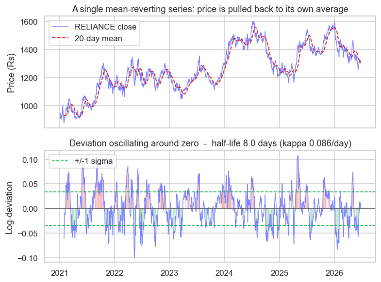
The top panel shows RELIANCE shadowing its own 20-day mean - never far, always pulled back. The bottom panel is the log-deviation oscillating around zero with one-sigma bands, the 8.0-day half-life annotated on it. The latest reading is +0.011, just above fair value, so no trade is live as this runs - the spring is barely stretched. Read it together and the picture is complete: a price that cannot be forecast in level, but whose distance from its average is forecastable enough to trade.

From one leash to two

The honest limitation of everything above is that truly reverting single series are rare. Most prices wander, and even our well-behaved deviation reverts only because we manufactured it from a moving average, which dulls the edge. The next chapter solves this properly. Instead of waiting for one price to behave, cointegration manufactures a reverting series from two assets - a synthetic spread engineered to mean-revert even when neither leg does on its own. It is the same OU machinery, the same kappa and the same half-life, simply applied to a spread rather than a single deviation, and it opens the door to market-neutral statistical arbitrage (Module G).

To recap:

• Prices are near random walks, but deviations, ratios and spreads can mean-revert - they have a home the price itself does not.
• The Ornstein-Uhlenbeck process models that pull: dx = kappa(theta - x)dt + sigma dW, with theta the mean, kappa the reversion speed, and sigma the noise. Discretised, it is an AR(1) model.
• Estimate kappa by regressing the daily change on the lagged level (slope = -kappa). For RELIANCE's deviation, kappa = 0.086 per day and the ADF test (p < 0.0001) confirms it truly reverts.
• The half-life ln(2)/kappa turns speed into time: 8.0 days here, which sets the holding period and a time-stop.
• Trade by z-scoring the deviation and fading extremes, but net the edge against costs, watch for regime breaks, and never leak the future when centring the series.

Next we take the same tools to two assets at once: cointegration and pairs trading.