Alternative Data and NLP for Indian Markets

Price and volume tell you what happened. Alternative data tries to tell you why, and sometimes before the tape does. A factory's satellite-lit night shift, a regulatory filing dropped at 6pm, a torrent of headlines about a weak monsoon - all of it is information that eventually moves a price, and the quant's hope is to read it a few minutes or a few hours early. This is the closing chapter of the alpha module, and deliberately so: alt data is the most seductive and the most treacherous edge in the book. The mechanics are easy to demo and brutally hard to turn into money. Let us do both - build a working text signal from scratch, then show you exactly where it breaks.

What counts as alternative data

Alternative data is anything that isn't the standard price, volume and open-interest feed your exchange broadcasts. The useful Indian-market buckets are:

• News and announcements: wire headlines, exchange corporate announcements, regulatory orders, monetary-policy statements.
• Filings and disclosures: quarterly results, shareholding patterns, insider-trading disclosures, bulk and block deal reports, the F&O ban list.
• Flow and positioning: FII and DII provisional figures, open-interest shifts (Chapter 64), delivery percentages.
• Genuinely exotic: satellite imagery, port and shipping data, app-download ranks, web traffic, credit-card panels.

Most of these arrive as text or as timestamped events, not tidy floating-point numbers. That is the whole game: turning unstructured language into a column you can line up next to returns. The discipline that does this is natural language processing, or NLP, and the simplest useful form is sentiment scoring.

From text to a number: the NLP pipeline

A text signal is a small assembly line. Raw text enters; a position-size exits. Every stage is replaceable - you can swap a lexicon for a transformer, or a simple average for a decay-weighted one - but the shape is always the same:

The tokeniser lowercases the text and splits it into words, throwing away punctuation. The sentiment stage scores those tokens - in its crudest form, by counting words from a positive list and a negative list and normalising the difference. The signal stage timestamps and aligns the score to a tradable bar (the dangerous step, as we will see). The position stage sizes it and passes it through your risk gates.

Let us build the first three stages on a handful of headlines and check them against the market. The lexicon and the headlines are defined inside the script - no paid feed - and the headlines are illustrative, but the NIFTY returns they are joined to are real:

# Score illustrative Indian-market headlines with a tiny lexicon, then join to the real same-day NIFTY return.
import os
from datetime import datetime

import numpy as np
import pandas as pd
from openalgo import api

client = api(
    api_key=os.getenv("OPENALGO_API_KEY", "your_api_key_here"),
    host=os.getenv("OPENALGO_HOST", "http://127.0.0.1:5000"),
)

# A minimal sentiment lexicon (the core of any bag-of-words NLP signal).
POS = {"surge", "beat", "rally", "gains", "strong", "cheer", "climb", "lifts",
       "upgrade", "inflows", "tops", "steady", "record", "buying", "optimism"}
NEG = {"plunge", "selloff", "weak", "slump", "hits", "cut", "fall", "miss",
       "downgrade", "fear", "outflows", "crash", "loss", "concern", "deepens"}

# Illustrative headlines, each tagged with a real trading date (the text is constructed for teaching).
HEADLINES = [
    ("2026-02-02", "RBI holds rates steady, signals strong growth; markets cheer"),
    ("2026-03-17", "FII inflows surge as rupee firms, banks rally on buying"),
    ("2026-04-07", "Earnings beat lifts IT majors, broad buying returns"),
    ("2026-05-12", "Global selloff deepens, weak monsoon fear hits sentiment, markets plunge"),
    ("2026-06-02", "Auto sales miss, profit booking caps gains, indices slump"),
    ("2026-06-24", "GDP tops estimates, demand outlook strong, indices climb"),
]


def score(text):
    tokens = "".join(ch.lower() if ch.isalnum() else " " for ch in text).split()
    pos = sum(t in POS for t in tokens)
    neg = sum(t in NEG for t in tokens)
    return (pos - neg) / max(pos + neg, 1)  # normalised to roughly [-1, +1]


# Real same-day NIFTY returns to provide price context for each dated headline.
end = datetime.now().strftime("%Y-%m-%d")
close = client.history(symbol="NIFTY", exchange="NSE_INDEX", interval="D",
                       start_date="2026-01-01", end_date=end)["close"]
ret = close.pct_change() * 100
ret.index = ret.index.strftime("%Y-%m-%d")

rows = []
print(f"{'date':<12}{'sentiment':>10}  {'NIFTY %':>8}  headline")
for date, text in HEADLINES:
    s = score(text)
    rmove = ret.get(date, np.nan)
    rows.append((s, rmove))
    print(f"{date:<12}{s:>+10.2f}  {rmove:>+8.2f}  {text[:54]}")

df = pd.DataFrame(rows, columns=["sent", "ret"]).dropna()
corr = df["sent"].corr(df["ret"])
print(f"\nToy sentiment-vs-same-day-return correlation over {len(df)} headlines: {corr:+.2f} "
      f"(real signals need thousands of dated items, not six).")

date         sentiment   NIFTY %  headline
2026-02-02       +1.00     +1.06  RBI holds rates steady, signals strong growth; markets
2026-03-17       +1.00     +0.74  FII inflows surge as rupee firms, banks rally on buyin
2026-04-07       +1.00     +0.68  Earnings beat lifts IT majors, broad buying returns
2026-05-12       -1.00     -1.83  Global selloff deepens, weak monsoon fear hits sentime
2026-06-02       -0.33     +0.43  Auto sales miss, profit booking caps gains, indices sl
2026-06-24       +1.00     +0.83  GDP tops estimates, demand outlook strong, indices cli

Toy sentiment-vs-same-day-return correlation over 6 headlines: +0.87 (real signals need thousands of dated items, not six).

The toy signal lines up startlingly well: a sentiment-versus-same-day-return correlation of +0.87 across the six headlines. That is exactly the kind of number that gets a research note written and a strategy funded. It is also almost entirely an illusion, and understanding why is the real lesson of this chapter. Six hand-picked headlines whose wording I chose are not a sample; they are a self-fulfilling prophecy. A real sentiment signal must be built from thousands of independently dated items, scored by a rule fixed before you ever see the returns. Shrink your sample and cherry-pick the text and you can manufacture any correlation you like.

Filings, announcements and the disclosure firehose

News is the loud channel; filings are the quiet, structured one, and often the richer. Indian listed companies disclose results, shareholding patterns, board outcomes, insider-trading windows and material events through the exchange announcement feed. Bulk and block deals (Chapter 24) are reported daily. The F&O ban list publishes overnight. Each of these is a clean, machine-readable event with a precise timestamp - which makes them far more tractable than free-form news.

The quant's job is to convert each disclosure into a feature: the surprise in a results number versus consensus, the change in promoter holding quarter on quarter, the direction of a block deal. The technique is the same pipeline - parse, score, align - but structured filings spare you most of the language ambiguity. A results PDF that says "profit after tax up 18%" needs a number extracted, not a mood inferred.

The two killers: look-ahead and sparsity

Two specific traps end most alt-data strategies before costs even get a vote.

Look-ahead bias is the assassin. A headline that hits the wire at 3:40pm cannot inform a trade at that day's 3:30pm close, yet it is trivially easy to join "today's sentiment" to "today's close return" in a dataframe and book a phantom edge. The red link in the figure is exactly this leak. The fix is iron discipline about timestamps: a signal may only use information strictly older than the bar it trades. If a results filing lands after hours, the earliest you can act is the next session's open. Get this wrong and your beautiful backtest is trading on tomorrow's newspaper.

Sparsity is the slower killer. A stock might have one genuine news event a month and nothing the other twenty-one trading days. So your signal is mostly blank, your sample of real events is tiny, and statistical significance is almost impossible to reach honestly (Chapter 13's multiple-testing problem bites hard here). Worse, the events cluster - results season, policy days - so the few observations you have are not even independent. Sparse, clustered, late-timestamped data is the natural habitat of the overfit.

A toy event study: do shocks drift?

If we cannot easily get a clean, dated news archive, we can use the market's own footprint of news as a proxy. A large overnight gap - the open jumping far from the prior close - usually means something happened while the market was shut: a result, an order, a global lead. An event study lines up many such shocks at a common "day zero" and averages the price path around them, asking the only question that matters for trading: after the shock, does the move continue (momentum, act on it) or reverse (overreaction, fade it)?

Here we detect every day SBIN gapped more than two percent in either direction over five years, orient each window in the gap's direction so the shocks add rather than cancel, and average the paths:

Copy

# Toy event study: detect large overnight-gap days (a proxy for news shocks) and plot the average price path around them.
import os
from datetime import datetime
from pathlib import Path

import matplotlib

matplotlib.use("Agg")
import matplotlib.pyplot as plt
import numpy as np
import seaborn as sns
from openalgo import api

client = api(
    api_key=os.getenv("OPENALGO_API_KEY", "your_api_key_here"),
    host=os.getenv("OPENALGO_HOST", "http://127.0.0.1:5000"),
)

SYM, EXCH, GAP, W = "SBIN", "NSE", 0.02, 10
end = datetime.now().strftime("%Y-%m-%d")
df = client.history(symbol=SYM, exchange=EXCH, interval="D",
                    start_date="2021-01-01", end_date=end).reset_index()
close = df["close"].values
gap = df["open"].values / np.roll(close, 1) - 1  # overnight gap vs prior close

# Event days: a large gap of either sign is our stand-in for an unscheduled news shock.
events = [i for i in range(W + 1, len(df) - W) if abs(gap[i]) > GAP]

# Build each window as cumulative return vs the close the day BEFORE the gap,
# then orient it in the direction of the gap so shocks add rather than cancel.
paths = []
for i in events:
    base = close[i - 1]
    path = (close[i - W: i + W + 1] / base - 1) * np.sign(gap[i]) * 100
    paths.append(path)
paths = np.array(paths)
offsets = np.arange(-W, W + 1)
mean_path = paths.mean(axis=0)
se = paths.std(axis=0) / np.sqrt(len(paths))

sns.set_theme(style="whitegrid")
fig, ax = plt.subplots(figsize=(8, 4.5))
ax.axvline(0, color="#888", ls="--", lw=1)
ax.fill_between(offsets, mean_path - se, mean_path + se, color="#7c83ff", alpha=0.2)
ax.plot(offsets, mean_path, color="#7c83ff", lw=1.8, marker="o", ms=3)
ax.set_title(f"{SYM}: average gap-oriented path around {len(events)} large-gap days (|gap| > {GAP:.0%})")
ax.set_xlabel("trading days from the gap (day 0)")
ax.set_ylabel("oriented return vs day -1 (%)")

out = Path(__file__).with_suffix(".png")
plt.savefig(out, dpi=110, bbox_inches="tight")
jump = mean_path[W] - mean_path[W - 1]      # day -1 close to day 0 close (the shock)
drift = mean_path[-1] - mean_path[W]        # day 0 close to day +10 close (after)
print(f"{SYM}: {len(events)} large-gap days. Mean shock day 0 = {jump:+.2f}%, "
      f"then drift to day +{W} = {drift:+.2f}%. Saved {out.name}")

Live output

SBIN: 33 large-gap days. Mean shock day 0 = +3.17%, then drift to day +10 = +0.68%. Saved 02_gap_event_study.png

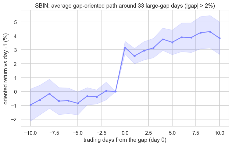
The picture is honest and humbling. Across 33 large-gap days, the average shock on day zero is +3.17% in the gap's direction - a large, real jump. But that jump happens at the open, before you can act on the information that caused it. What is left to trade is the drift afterward, and it averages just +0.68% over the following ten sessions, with a wide error band straddling zero. So the news was real and the move was real, but the tradable residue - the part you can capture once the gap has already printed - is small, noisy, and very likely smaller than the round-trip cost of chasing it. That gap between "the news mattered" and "I could have made money from the news" is the entire difficulty of alt-data alpha in one chart.

Alt data and NLP are not magic, and they are not fraud - they are simply the hardest place to be honest. The pipeline is easy: tokenise, score, align, size. The edge is hard, because the same properties that make text valuable (it is unstructured, sparse and freshly timestamped) are exactly the properties that invite look-ahead and overfitting. Treat every text signal as guilty until a clean, out-of-sample, properly-timestamped test proves it innocent, and you will discard ninety-five ideas to keep one worth trading.

That instinct - guilty until proven innocent - is the bridge to the next module. We have spent Module G finding edges: the research process, statistical arbitrage, flow, intraday models, and now text. Module H is where we stop trusting them. Backtesting done right, look-ahead and survivorship audits, walk-forward and purged cross-validation, machine learning without leakage, and portfolio construction that turns many fragile signals into one survivable book. The alpha is found; now we find out whether any of it was ever real.

Recap

• Alternative data is anything beyond price, volume and OI: news, filings, flow and the genuinely exotic - mostly arriving as text or timestamped events.
• The text-signal pipeline is tokenise, score sentiment, align to a timestamp, size a position - each stage swappable.
• Our toy lexicon scored a +0.87 correlation to same-day NIFTY returns on six headlines, which is a manufactured illusion, not an edge - real signals need large, independently dated corpora.
• Look-ahead (trading on information you only had later) and sparsity (too few, clustered, late events) kill most alt-data strategies before costs do.
• An event study on SBIN's 33 large-gap days showed a +3.17% day-zero shock but only +0.68% of tradable drift over ten days - the news was real, the residual edge was thin.