Impact Cost, Slippage and Transaction Cost Analysis

Your strategy decides to buy at 6570. By the time the order is done, your average price is 6572.70. Nobody moved the market against you out of malice - you did, by demanding more liquidity than was resting at the touch. That 2.70 you gave up is not brokerage, not STT, not even the spread alone. It is market impact, and it is the single cost that most cleanly separates a backtest from a brokerage statement. Chapter 25 measured how thin a market is. This chapter prices what that thinness costs you when you actually trade, and shows how professionals account for it honestly.

Two kinds of impact: temporary and permanent

When you push a large buy through, the price reacts in two distinct ways, and a quant must keep them apart.

• Temporary impact is the price you pay to consume resting liquidity right now. You walk up the ask staircase, the book is dented, and once your order finishes the patient sellers return and the price relaxes back toward where it was. This is a liquidity premium - rent you pay for immediacy. It is yours alone, and a patient trader avoids most of it.
• Permanent impact is the part of the move that stays. The market reads your relentless buying as information - someone knows something - and re-prices upward for good. This is the cost of revealing your hand. You cannot trade your way out of it by slowing down; you only reduce it by being harder to detect.

The split matters because the two respond to opposite tactics. Temporary impact shrinks when you trade slower and smaller. Permanent impact shrinks when you trade quieter - smaller child orders, randomised timing, more passive fills. Confuse the two and you optimise the wrong knob.

This is where Kyle's lambda from Chapter 25 earns its keep. Lambda is the slope of permanent impact against signed order flow: price moves by lambda times net quantity traded. A deep name has a tiny lambda; a thin one a large lambda. Permanent impact is essentially lambda multiplied by the size you reveal to the market.

Slippage, arrival price and implementation shortfall

"Slippage" gets thrown around loosely, so pin it to a benchmark. Slippage is the difference between the price you expected and the price you got - but expected against what? The honest benchmark is the arrival price (also called the decision price): the mid-quote at the instant your strategy decided to trade. Everything that happens between that decision and your last fill is your execution cost, and none of it can hide.

Andre Perold gave this its proper name in 1988: implementation shortfall - the gap between a "paper portfolio" that trades instantly and free at the arrival price, and the real portfolio you actually end up holding. It bundles every leak into one number: the spread you crossed, the impact you caused, the drift while you waited, and the opportunity cost of any quantity you failed to fill. It is the most honest single figure in execution precisely because it hides nothing.

Contrast it with the popular VWAP benchmark (the volume-weighted average price over your trading window). Beating VWAP feels good, but VWAP is a moving target you partly create: trade passively all day and you roughly match VWAP by construction, even if the arrival-to-close drift quietly cost you a fortune. VWAP measures whether you executed in line with the crowd; implementation shortfall measures whether trading made money versus the idea. A quant cares about the second.

Walking the book: impact you can compute

You do not need a model to see temporary impact - it is sitting in the order book. A market buy fills against the best ask, then the next level, then the next, each worse than the last, so your average fill drifts above the mid. Summing price times quantity up the ladder until the order is full gives you the exact cost, level by level.

# Walk a real L5 order book to price the market-impact cost of a sized market order.
import os

from openalgo import api

client = api(
    api_key=os.getenv("OPENALGO_API_KEY", "your_api_key_here"),
    host=os.getenv("OPENALGO_HOST", "http://127.0.0.1:5000"),
)

# Prefer a live book: MCX near-month future (trades into the night), then a liquid NSE name.
CANDIDATES = [("CRUDEOIL20JUL26FUT", "MCX"), ("RELIANCE", "NSE"), ("SBIN", "NSE")]
ORDER_QTY = 40  # units to BUY at market (lots for the future, shares for the stock)


def resolve_book(cands):
    # Use the first candidate whose live L5 has real prices and quantities on both sides.
    for sym, exch in cands:
        d = client.depth(symbol=sym, exchange=exch).get("data", {})
        asks = [a for a in d.get("asks", []) if a["price"] > 0 and a["quantity"] > 0]
        bids = [b for b in d.get("bids", []) if b["price"] > 0 and b["quantity"] > 0]
        if asks and bids:
            return sym, exch, bids, asks, float(d["ltp"]), True
    # Off-hours the book is empty: reconstruct an illustrative ladder around the REAL last price.
    sym, exch = cands[0]
    ltp = float(client.depth(symbol=sym, exchange=exch)["data"]["ltp"])
    profile = [6, 10, 14, 20, 30]  # a typical thinning depth profile
    asks = [{"price": ltp + i, "quantity": q} for i, q in enumerate(profile, start=1)]
    bids = [{"price": ltp - i, "quantity": q} for i, q in enumerate(profile, start=1)]
    return sym, exch, bids, asks, ltp, False


sym, exch, bids, asks, ltp, is_live = resolve_book(CANDIDATES)
mid = (bids[0]["price"] + asks[0]["price"]) / 2

# Walk the ASK side: fill the buy order level by level until the size is met.
need, cost, filled = ORDER_QTY, 0.0, 0
for lvl in asks:
    take = min(need, lvl["quantity"])
    cost += take * lvl["price"]
    filled, need = filled + take, need - take
    if need <= 0:
        break

avg_fill = cost / filled
impact_bps = (avg_fill - mid) / mid * 1e4
half_spread_bps = (asks[0]["price"] - mid) / mid * 1e4
walk_bps = impact_bps - half_spread_bps

tag = "LIVE book" if is_live else "live book CLOSED - illustrative ladder around real LTP"
print(f"{sym} ({exch})  {tag}  mid {mid:.2f}")
print(f"Market buy {filled}/{ORDER_QTY} units -> avg fill {avg_fill:.2f} vs mid {mid:.2f}")
print(f"Impact {avg_fill - mid:.2f} = {impact_bps:.1f} bps "
      f"({half_spread_bps:.1f} bps half-spread + {walk_bps:.1f} bps walking the book)")

CRUDEOIL20JUL26FUT (MCX)  live book CLOSED - illustrative ladder around real LTP  mid 6570.00
Market buy 40/40 units -> avg fill 6572.70 vs mid 6570.00
Impact 2.70 = 4.1 bps (1.5 bps half-spread + 2.6 bps walking the book)

On the latest near-month crude oil future, a market buy of 40 lots fills at an average of 6572.70 against a mid of 6570.00 - an impact of 2.70, or 4.1 basis points. Of that, 1.5 bps is simply crossing the half-spread and 2.6 bps is the walk up the staircase. (When the market is shut the script reconstructs an illustrative ladder around the real last price; run it during the session and it walks the genuine live book exactly the same way.) Notice the structure: the spread-crossing cost is roughly fixed per trade, but the walk-up grows with your size. Double the order and the half-spread cost is unchanged while the staircase bites deeper.

The square-root law

Walking the book prices one snapshot, but you need impact before you trade, as a function of size. The most robust empirical regularity in all of execution is the square-root law: impact grows not linearly with size but with its square root. Doubling your order multiplies impact by about 1.4, not 2. Formally, cost in volatility units is roughly Y times sigma times the square root of participation - your order divided by average daily volume (ADV) - where Y is a constant near 0.5 and sigma is daily volatility. This shape recurs across decades of data, asset classes and venues (documented by Almgren, Bouchaud and colleagues), which is why it survives where prettier linear models fail.

Copy

# The square-root law: impact grows with the square root of participation (order / ADV).
import os
from datetime import datetime, timedelta
from pathlib import Path

import matplotlib

matplotlib.use("Agg")
import matplotlib.pyplot as plt
import numpy as np
import seaborn as sns
from openalgo import api

client = api(
    api_key=os.getenv("OPENALGO_API_KEY", "your_api_key_here"),
    host=os.getenv("OPENALGO_HOST", "http://127.0.0.1:5000"),
)

SYMBOL, EXCHANGE = "RELIANCE", "NSE"
end = datetime.now().strftime("%Y-%m-%d")
start = (datetime.now() - timedelta(days=365)).strftime("%Y-%m-%d")
df = client.history(symbol=SYMBOL, exchange=EXCHANGE, interval="D", start_date=start, end_date=end)

adv = df["volume"].tail(20).mean()                  # average daily volume, shares (real)
price = float(df["close"].iloc[-1])                 # latest close (real)
sigma_bps = df["close"].pct_change().std() * 1e4    # daily volatility in bps (real)
Y = 0.5                                             # calibration constant (square-root prefactor)

# Impact curve: cost(bps) = Y * sigma * sqrt(participation), participation = order / ADV.
part = np.logspace(-5, np.log10(0.30), 200)         # 0.001% to 30% of ADV
impact_bps = Y * sigma_bps * np.sqrt(part)

# A realistic active-retail order in rupees, expressed as a fraction of ADV.
retail_rs = 10_00_000
retail_part = (retail_rs / price) / adv
retail_impact = Y * sigma_bps * np.sqrt(retail_part)
inst_impact = Y * sigma_bps * np.sqrt(0.05)         # an institutional 5%-of-ADV order

sns.set_theme(style="whitegrid")
fig, ax = plt.subplots(figsize=(8, 4.5))
ax.plot(part * 100, impact_bps, color="#7c83ff", lw=2, label="square-root impact")
ax.scatter([retail_part * 100], [retail_impact], color="#16a34a", zorder=5,
           label=f"Rs 10L retail ({retail_part * 100:.4f}% ADV)")
ax.axvline(5, color="#dc2626", ls="--", lw=1.2, label="5% ADV (institutional)")
ax.set_xscale("log")
ax.set_title(f"{SYMBOL} - square-root impact (sigma {sigma_bps:.0f} bps/day, ADV {adv / 1e6:.1f}M sh)")
ax.set_xlabel("Order size as % of ADV (log scale)")
ax.set_ylabel("Estimated impact (bps)")
ax.legend()

out = Path(__file__).with_suffix(".png")
plt.savefig(out, dpi=110, bbox_inches="tight")
print(f"ADV {adv / 1e6:.1f}M sh, sigma {sigma_bps:.0f} bps/day. "
      f"Rs 10L retail = {retail_part * 100:.4f}% ADV -> ~{retail_impact:.2f} bps; "
      f"5% ADV -> ~{inst_impact:.0f} bps. Saved {out.name}")

Live output

ADV 18.2M sh, sigma 131 bps/day. Rs 10L retail = 0.0042% ADV -> ~0.42 bps; 5% ADV -> ~15 bps. Saved 02_sqrt_impact.png

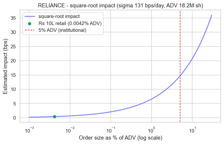
Calibrated on Reliance with a real 131 bps-per-day volatility and a 20-day ADV of 18.2 million shares, the curve is brutally instructive. A Rs 10 lakh retail order is about 0.0042% of ADV and costs roughly 0.42 bps of impact - utterly negligible, smaller than a single tick. The same model says a 5%-of-ADV institutional order costs about 15 bps: thirty-five times more impact for a far larger trade. That is the square root at work, and it is the central reason capacity is finite - an edge of 10 bps per trade is pure profit at retail size and entirely eaten by impact at fund size.

Honest transaction cost analysis

Transaction cost analysis (TCA) is the discipline of measuring all of this on your real fills and feeding it back into the strategy. Done honestly it compares every fill to its arrival price, decomposes the shortfall into spread, impact and drift, and reports it net of brokerage, STT and exchange charges. Done dishonestly it picks VWAP as the benchmark, ignores unfilled quantity, and quietly drops the days the algorithm misbehaved.

India gives you an unusually clean anchor for this. NSE makes impact cost its official measure of liquidity: the NSE Indices methodology document defines impact cost as the percentage degradation from mid for a specified order value, and a stock qualifies for the Nifty 50 only if its average impact cost stays at or below 0.50% for that basket (the basket value is set by NSE and revised periodically). In other words, the exchange itself certifies index membership using exactly the book-walk you ran above - a real, computable number, consistent with NSE's published microstructure research on spreads and the limit order book.

Impact is the cost that scales with you; TCA is how you keep yourself honest about it. With the cost of trading now properly priced, the next chapter turns to the information in trading - reading volume, open interest and order flow to infer who is pushing the price, and whether they know something you do not.