Forecast Evaluation and Model Decay

Every quant eventually owns a model that used to work. It backtested beautifully, it traded well for a while, and then - quietly, without an announcement - it stopped. No crash, no blown-up account, just a slow bleed where the win rate slid toward a coin flip and the equity curve went flat. The hard part was never building the forecast. The hard part is knowing, honestly and early, how good it is, whether that goodness is real, and when it has died. That is what this chapter is about: scoring forecasts, separating skill from luck, and detecting decay before it empties your account.

Scoring a forecast: error and direction

A forecast makes a number; reality makes another. The gap between them is what we score, and there are two families of scores that matter to a trader.

The first family measures magnitude error - how far off the number was. Mean squared error (MSE) averages the squared gaps, mean((forecast - actual)^2); its square root, RMSE, is back in the original units (say, percent). Mean absolute error (MAE) averages the absolute gaps, mean(|forecast - actual|). MSE punishes large misses far more harshly than small ones because of the square, so a model that is usually close but occasionally wild scores worse on MSE than on MAE. Use MSE when big errors are genuinely costly; use MAE when you want a robust, outlier-tolerant read.

The second family measures direction - did you get the sign right? Directional accuracy (or hit rate) is simply the fraction of days the forecast called up-versus-down correctly. For a trader this is often the metric that pays, because a position keyed off the sign earns money whenever the sign is right, regardless of whether the magnitude was perfect.

There is a trap hiding in error metrics, and it is worth naming now. RMSE and MAE are not comparable across different volatility regimes. A calm year produces small returns and therefore small errors, so a model can look more accurate simply because the market got quieter, not because the model got smarter. The fix is to benchmark against a naive forecast (predict the mean, or predict zero) and report the improvement, not the raw number. A model that cannot beat "predict the average" has no skill, however small its RMSE looks.

In-sample is a salesman, out-of-sample is the auditor

Here is the single most expensive mistake in quantitative trading: judging a model on the same data you used to build it. Any model with enough freedom can fit the past. Fitting the past is not a forecast; it is memorisation. The only score that means anything is the one earned on data the model never saw while it was being chosen.

So we split the history. The early slice is in-sample - the model is allowed to learn here. The later slice is out-of-sample - sacred, untouched, the auditor's data. We score on the out-of-sample slice and treat that, and only that, as the truth.

# Backtest a momentum-sign forecast on NIFTY, split in-sample vs out-of-sample, and measure the decay.
import os
from datetime import datetime

import numpy as np
import pandas as pd
from openalgo import api
from scipy import stats

client = api(
    api_key=os.getenv("OPENALGO_API_KEY", "your_api_key_here"),
    host=os.getenv("OPENALGO_HOST", "http://127.0.0.1:5000"),
)

end = datetime.now().strftime("%Y-%m-%d")
close = client.history(symbol="NIFTY", exchange="NSE_INDEX", interval="D",
                       start_date="2015-01-01", end_date=end)["close"].astype(float)

# Forecast: sign of (20-day SMA minus 50-day SMA), shifted, predicts tomorrow's direction.
ret = close.pct_change()
sig = np.sign(close.rolling(20).mean() - close.rolling(50).mean()).shift(1)
df = pd.DataFrame({"ret": ret, "sig": sig}).dropna()
df = df[df.sig != 0]

hit = (np.sign(df.ret) == df.sig).astype(int)          # 1 if direction called right
split = int(len(df) * 0.65)                              # first 65% = in-sample
ins, oos = hit.iloc[:split], hit.iloc[split:]


def assess(h):
    p, n = h.mean(), len(h)
    z = (p - 0.5) / np.sqrt(0.25 / n)                    # is the edge over 50% real?
    return p, n, z, 1 - stats.norm.cdf(z)


pi, ni, zi, pvi = assess(ins)
po, no, zo, pvo = assess(oos)
ann = lambda h: (df.sig * df.ret).loc[h.index].mean() * 252 * 100

print(f"20/50 momentum-sign forecast on NIFTY, split {df.index[split].date()}")
print(f"{'':22s}{'in-sample':>14s}{'out-of-sample':>16s}")
print(f"{'directional accuracy':22s}{pi*100:>13.2f}%{po*100:>15.2f}%")
print(f"{'miss rate (error)':22s}{(1-pi)*100:>13.2f}%{(1-po)*100:>15.2f}%")
print(f"{'edge over coin flip':22s}{(pi-0.5)*100:>+12.2f}pt{(po-0.5)*100:>+14.2f}pt")
print(f"{'z vs 50%':22s}{zi:>14.2f}{zo:>16.2f}")
print(f"{'p-value (one-sided)':22s}{pvi:>14.4f}{pvo:>16.4f}")
print(f"{'ann. signed return':22s}{ann(ins):>13.2f}%{ann(oos):>15.2f}%")
print(f"\nEdge real in-sample (p={pvi:.4f}); out-of-sample it is a coin flip (p={pvo:.3f}) - the model decayed.")

20/50 momentum-sign forecast on NIFTY, split 2022-07-14
                           in-sample   out-of-sample
directional accuracy          53.19%          51.53%
miss rate (error)             46.81%          48.47%
edge over coin flip          +3.19pt         +1.53pt
z vs 50%                        2.72            0.96
p-value (one-sided)           0.0032          0.1687
ann. signed return            11.70%           3.92%

Edge real in-sample (p=0.0032); out-of-sample it is a coin flip (p=0.169) - the model decayed.

The result is sobering and typical. A simple 20-over-50-day momentum-sign forecast on NIFTY calls tomorrow's direction right 53.19% of the time in-sample but only 51.53% out-of-sample. The miss rate (the directional error) rises from 46.81% to 48.47%. The edge over a coin flip is more than halved, from +3.19 points to +1.53 points. And the money tracks it: the signal earns an annualised 11.70% in the period where it was measured, then just 3.92% out-of-sample. The model did not break. It simply returned closer to its honest, much smaller true edge once it was tested on data it could not have been tuned to.

Is the difference real, or just luck?

A 53% hit rate sounds like an edge. But over a few hundred days, 53% could easily be the random scatter of a fair coin. Before you trade a number, you must ask whether it is statistically distinguishable from chance. This is the spirit of the Diebold-Mariano test.

Diebold-Mariano compares two forecasts by looking at the difference in their losses day by day - for instance, model A's squared error minus a benchmark's squared error. If that loss-differential series has a mean reliably below zero, model A genuinely forecasts better; if its mean is statistically indistinguishable from zero, the apparent improvement is noise. The key insight is that you are not comparing the headline accuracy numbers, you are testing whether the gap between them survives the uncertainty of a finite sample.

The example applies the same logic to direction. It runs a proportion test asking "is this hit rate really above 50%?" In-sample, the edge clears the bar easily: a z-statistic of 2.72 and a one-sided p-value of 0.0032, comfortably significant. Out-of-sample, the same test returns a z of 0.96 and a p-value of 0.169 - nowhere near significance. In plain words: in the data we fitted on, the edge looks real; in the data that matters, it is statistically a coin flip.

The half-life of an edge

Even a model that passes every test on launch day is living on borrowed time. Edges decay. Other traders find the same pattern and arbitrage it away; the market regime that birthed the signal gives way to another; the crowd that made momentum work piles in until it whipsaws. A live model's accuracy is not a constant - it is a slowly falling curve, and your job is to watch it fall.

The practical tool is a rolling hit rate - the model's directional accuracy computed over a moving window (a year, say) and plotted through time. A healthy edge hovers above the 50% line; a dying one sags toward it and eventually crosses below, where the signal is not merely useless but actively wrong.

Copy

# Plot the rolling 1-year out-of-sample hit rate of a momentum signal decaying toward the coin-flip line.
import os
from datetime import datetime
from pathlib import Path

import matplotlib

matplotlib.use("Agg")
import matplotlib.pyplot as plt
import numpy as np
import pandas as pd
import seaborn as sns
from openalgo import api

client = api(
    api_key=os.getenv("OPENALGO_API_KEY", "your_api_key_here"),
    host=os.getenv("OPENALGO_HOST", "http://127.0.0.1:5000"),
)

end = datetime.now().strftime("%Y-%m-%d")
close = client.history(symbol="NIFTY", exchange="NSE_INDEX", interval="D",
                       start_date="2015-01-01", end_date=end)["close"].astype(float)

ret = close.pct_change()
sig = np.sign(close.rolling(20).mean() - close.rolling(50).mean()).shift(1)
df = pd.DataFrame({"ret": ret, "sig": sig}).dropna()
df = df[df.sig != 0]

hit = (np.sign(df.ret) == df.sig).astype(int)
roll = hit.rolling(252).mean()                 # rolling 1-year directional hit rate
ins_level = hit.iloc[:int(len(df) * 0.65)].mean()

sns.set_theme(style="whitegrid")
fig, ax = plt.subplots(figsize=(10, 4.6))
ax.plot(roll.index, roll * 100, color="#7c83ff", lw=1.6, label="rolling 1-year hit rate")
ax.axhline(50, color="#dc2626", ls="--", lw=1.3, label="coin flip (50%)")
ax.axhline(ins_level * 100, color="#16a34a", ls=":", lw=1.3, label=f"early edge ({ins_level*100:.1f}%)")
ax.fill_between(roll.index, 50, roll * 100, where=(roll * 100 >= 50), color="#16a34a", alpha=0.08)
ax.fill_between(roll.index, 50, roll * 100, where=(roll * 100 < 50), color="#dc2626", alpha=0.08)
ax.set_title("NIFTY 20/50 momentum sign: the edge bleeds back to a coin flip")
ax.set_ylabel("directional hit rate (%)")
ax.set_ylim(38, 70)
ax.legend(loc="upper right", fontsize=9)

fig.tight_layout()
out = Path(__file__).with_suffix(".png")
plt.savefig(out, dpi=110, bbox_inches="tight")
print(f"Rolling hit rate fell from a {roll.max()*100:.1f}% peak to {roll.dropna().iloc[-1]*100:.1f}% recently "
      f"(coin flip is 50%). Saved {out.name}")

Live output

Rolling hit rate fell from a 65.1% peak to 42.5% recently (coin flip is 50%). Saved 02_rolling_hitrate.png

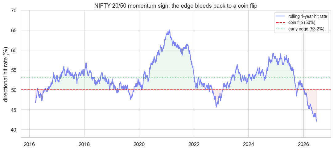
The picture is unforgiving. The same NIFTY momentum signal had a rolling one-year hit rate that peaked at 65.1% in its glory days, then bled steadily lower until, in the most recent window, it sits at 42.5% - below the coin flip. An edge that looked structural in 2020 and 2021 has not just faded, it has inverted in the recent chop. Anyone still trading it on faith, without watching this curve, is paying for a pattern the market stopped honouring.

When to retire a model

Knowing a model is decaying is useless without a rule for acting on it, decided in advance while you are calm. Retire-or-review triggers worth committing to before you ever go live:

• Significance lost. The rolling out-of-sample edge can no longer beat a coin flip at your chosen confidence (the Diebold-Mariano or proportion test stops clearing). The edge is now indistinguishable from luck.
• Drawdown beyond design. Live losses exceed the worst the backtest ever produced. The world the model assumed no longer holds.
• Regime break. A structural change - a new market microstructure rule, a volatility regime shift, a crowding-out by copycats - invalidates the premise the signal was built on.
• Capacity exhaustion. The edge survives but is too small to cover costs at the size you must trade, which is the subject of the next chapter.

The discipline of this chapter is the discipline of honesty: score on out-of-sample data, demand statistical significance, watch the rolling accuracy, and pre-commit to retirement rules. Do that and you will lose models gracefully instead of losing accounts violently. Next we make the cost side precise - how turnover, market impact and a signal's half-life set the ceiling on how much capital an edge can actually carry before it eats itself.