HFT vs Algo Trading vs Systematic Trading
Three words people confuse - the latency, holding period and infrastructure that separate true HFT from algorithmic and systematic trading.
- ·Defining HFT
- ·Algo vs systematic
- ·Latency and holding periods
- ·Who can play at each level
- ·Infrastructure by tier
- ·Where retail quants fit
Three phrases get thrown around as if they were the same thing: algorithmic trading, systematic trading and high-frequency trading. A newcomer hears all three and pictures one image - a fast computer beating humans to the trade. They are not the same thing, and confusing them is the single most expensive misunderstanding a new quant can carry. One of these words describes how an order reaches the market. One describes how a decision gets made. Only one is about raw speed - and it is the one you will never compete on, and never need to. Getting these three straight tells you exactly which game is open to you, and which one to ignore.
Three words that are not synonyms
Algorithmic trading is the broadest term. It means a computer, following rules, decides or places orders without a human approving each one. That is the entire definition. It says nothing about speed and nothing about holding period. A program that rebalances a portfolio once a month is algo trading; so is a market-making engine that quotes ten thousand times a second. Algo is the umbrella, and everything in this module lives under it.
Systematic trading is a philosophy of decision-making. Every entry, exit and size follows a pre-defined, testable rule or model rather than a gut feeling. Its opposite is discretionary trading, where a human applies judgement. Systematic is about rules versus intuition, not about speed. A systematic fund might hold a position for three weeks; what makes it systematic is that a model, not a mood, chose the trade. Almost all systematic trading is implemented as algo trading, but its defining feature is the research discipline behind it.
High-frequency trading (HFT) is a narrow subset of algo trading, defined purely by speed and frequency: holding periods of milliseconds to seconds, latency measured in microseconds, order counts in the tens of thousands per day, and an edge that comes mostly from being first. HFT is always algorithmic and almost always systematic, but the reverse is emphatically false. The vast majority of algorithmic and systematic trading is nowhere near high frequency.
"Algo" answers is a human in the loop? "Systematic" answers rules or judgement? "HFT" answers how fast and how often? They are three different questions, not three points on one line. A retail quant should aim to be algorithmic and systematic, and has no business being high-frequency.
The axes that actually separate them
Stop picturing these as three dots on a single ruler. They differ along several axes at once, and the table below is the honest map.
| HFT | Intraday algo | Systematic | |
|---|---|---|---|
| Latency that matters | microseconds | tens of ms | seconds, irrelevant |
| Holding period | ms to seconds | minutes to hours | days to months |
| Trades per day | tens of thousands | tens | a fraction |
| Infrastructure | colocation, tick feed | cloud server, fast API | a laptop, daily data |
| Source of edge | speed, queue position | short-term signal | research depth, patience |
| Capital to enter | crores | modest | small |
Notice that latency - the obsession of the next chapter - only bites at the top tier. By the time your holding period is a day, being ten milliseconds faster is worth precisely nothing. That single fact is the door retail walks through.
Horizons in numbers
Words are slippery; numbers are not. The first example pulls real NIFTY history at two scales - one-minute bars and daily bars - and measures how large a typical move is, and how often a simple trend signal fires, at each.
# Horizons in numbers: typical move size and signal frequency at minute vs day scale.
import os
from datetime import datetime, timedelta

import numpy as np
from openalgo import api, ta

client = api(
    api_key=os.getenv("OPENALGO_API_KEY", "your_api_key_here"),
    host=os.getenv("OPENALGO_HOST", "http://127.0.0.1:5000"),
)

end = datetime.now().strftime("%Y-%m-%d")
SYM, EXCH = "NIFTY", "NSE_INDEX"


def horizon(interval, start):
    df = client.history(symbol=SYM, exchange=EXCH, interval=interval,
                        start_date=start, end_date=end)
    c = df["close"]
    r = np.log(c / c.shift(1)).dropna()
    move_bps = r.abs().median() * 1e4                          # typical move per bar (bps)
    rng_bps = ((df["high"] - df["low"]) / c).median() * 1e4    # typical bar range (bps)
    sig = np.sign(ta.ema(c, 9) - ta.ema(c, 21))                # a simple trend signal
    sig = sig[~np.isnan(sig)]
    flips = int((np.diff(sig) != 0).sum())                     # crossover signals fired
    n_days = df.index.normalize().nunique()
    bars_per_day = len(df) / n_days
    sig_per_day = flips / n_days
    hold_bars = len(df) / flips                                # avg bars held per trade
    return dict(move_bps=move_bps, rng_bps=rng_bps, std=r.std(),
                bars_per_day=bars_per_day, sig_per_day=sig_per_day, hold_bars=hold_bars)


m = horizon("1m", (datetime.now() - timedelta(days=20)).strftime("%Y-%m-%d"))
d = horizon("D", "2021-01-01")

print(f"NIFTY horizons in numbers\n{'-' * 58}")
print(f"{'':12}{'minute bar':>14}{'daily bar':>14}")
print(f"{'typ move':12}{m['move_bps']:>11.1f} bps{d['move_bps'] / 100:>11.2f} %")
print(f"{'typ range':12}{m['rng_bps']:>11.1f} bps{d['rng_bps'] / 100:>11.2f} %")
print(f"{'bars/day':12}{m['bars_per_day']:>14.0f}{d['bars_per_day']:>14.0f}")
print(f"{'signals/day':12}{m['sig_per_day']:>14.2f}{d['sig_per_day']:>14.3f}")
print(f"{'~hold/trade':12}{m['hold_bars']:>9.0f} min{d['hold_bars']:>10.0f} days")

ratio = d["std"] / m["std"]
print(f"{'-' * 58}\nDaily vol is {ratio:.0f}x minute vol (sqrt(375) rule says {np.sqrt(375):.0f}x).")
print(f"Minute scale: tiny ~{m['move_bps']:.1f} bps moves, ~{m['bars_per_day']:.0f} a day - "
      f"the high-frequency end (HFT goes finer still, sub-second).")
print(f"Day scale: a fat ~{d['move_bps'] / 100:.2f} % move once a day, signal flips every "
f"~{d['hold_bars']:.0f} days - the systematic end.")NIFTY horizons in numbers
----------------------------------------------------------
minute bar daily bar
typ move 1.4 bps 0.50 %
typ range 3.1 bps 0.91 %
bars/day 375 1
signals/day 16.00 0.043
~hold/trade 23 min 23 days
----------------------------------------------------------
Daily vol is 23x minute vol (sqrt(375) rule says 19x).
Minute scale: tiny ~1.4 bps moves, ~375 a day - the high-frequency end (HFT goes finer still, sub-second).
Day scale: a fat ~0.50 % move once a day, signal flips every ~23 days - the systematic end.The output is stark. A one-minute NIFTY bar moves a median of 1.4 basis points, with a high-low range of about 3.1 bps. A daily bar moves about 0.50%, with a 0.91% range. The daily move is roughly 23 times the minute move, almost exactly the square-root-of-time scaling that volatility obeys (the square root of 375 minutes is about 19). There are 375 one-minute bars in a NIFTY session and just one daily bar. So the minute world offers tiny moves but hundreds of chances a day; the daily world offers one fat move you must wait the whole session for.
That is the entire logic of the speed spectrum in one table. To make a living off a 1.4 bp move you must trade it thousands of times, with costs near zero and latency near zero - that is HFT, and it works at scales far finer than one minute, down to sub-second ticks. To make a living off a 0.50% daily move you only need to be right and patient a handful of times a month - that is systematic trading, and it does not care who is faster.
Volatility scaling with the square root of time is why the horizons feel so different. Stretching risk over a day instead of a minute multiplies the available move by about 19, but it multiplies the wait too. Speed buys you frequency; horizon buys you size. You cannot have both at once.
Who can actually play at each tier
The tiers are gated by capital and infrastructure, not by talent.
HFT requires renting rack space inside the exchange's own data centre (colocation), specialised network cards, a tick-by-tick data feed and a team of engineers. Entry costs run to crores per year before a single rupee of profit. The edge is mechanical and physical, and the next chapter shows exactly why no laptop can ever close that gap.
Intraday algo trading sits in the middle. A cloud server near the broker, a reasonably fast API and intraday data are enough to run it. The barrier is not crores; it is the brutal arithmetic of costs. From the example, an intraday signal that flips position around 16 times a day pays the spread and charges sixteen times daily - and against a 1.4 bp move, those costs eat most setups alive. Most retail intraday algos lose not to a smarter opponent but to their own turnover.
Systematic trading is wide open. The infrastructure is a laptop, historical data and an order gateway such as OpenAlgo talking to a broker API. The edge comes from research depth and discipline, the very axes HFT cannot buy. Holding for days or weeks makes latency, colocation and tick feeds all irrelevant.
The middle tier is a trap for the underfunded. Intraday algo trading looks reachable because you can code it on a laptop, yet it competes closest to the firms that genuinely are fast, and its high turnover makes it the most cost-sensitive game retail can play. Do not mistake "I can run it" for "I can win at it."
Where you actually fit
Plotting the three tiers on one map makes the choice obvious. The second example places each on a log-log chart of holding period against trades per day, measuring the two retail-reachable points from real NIFTY data and marking HFT from published figures.
# A log-log map of the three tiers: holding period vs trades per day.
# The two retail-reachable points are measured from real NIFTY data; HFT is a labelled reference.
import os
from datetime import datetime, timedelta
from pathlib import Path

import matplotlib

matplotlib.use("Agg")
import matplotlib.pyplot as plt
import numpy as np
import seaborn as sns
from openalgo import api, ta

client = api(
    api_key=os.getenv("OPENALGO_API_KEY", "your_api_key_here"),
    host=os.getenv("OPENALGO_HOST", "http://127.0.0.1:5000"),
)

end = datetime.now().strftime("%Y-%m-%d")


def tier(interval, start, sec_per_bar):
    df = client.history(symbol="NIFTY", exchange="NSE_INDEX", interval=interval,
                        start_date=start, end_date=end)
    c = df["close"]
    sig = np.sign(ta.ema(c, 9) - ta.ema(c, 21))
    sig = sig[~np.isnan(sig)]
    flips = int((np.diff(sig) != 0).sum())
    n_days = df.index.normalize().nunique()
    trades_per_day = flips / n_days
    hold_sec = (len(df) / flips) * sec_per_bar       # avg bars held -> seconds
    return hold_sec, trades_per_day


# Two REAL points from data: an intraday algo (1m) and a systematic book (daily).
intraday = tier("1m", (datetime.now() - timedelta(days=20)).strftime("%Y-%m-%d"), 60)
systematic = tier("D", "2018-01-01", 86400)          # a daily position is held over calendar days
# One REFERENCE point: HFT colocated - typical published figures, not retail-measurable.
hft = (1e-3, 5e4)                                     # ~1 ms holds, tens of thousands of trades/day

pts = [("HFT (colocated)\nmicroseconds-ms", hft, "#dc2626"),
       ("Intraday algo\n(1m EMA cross)", intraday, "#7c83ff"),
       ("Systematic\n(daily trend)", systematic, "#16a34a")]

sns.set_theme(style="whitegrid")
fig, ax = plt.subplots(figsize=(8.5, 5.5))
xs = np.array([p[1][0] for p in pts])
ax.plot(xs, 1.0 / xs * 86400, color="#9a9a9a", lw=1, ls="--", alpha=0.6,
        label="trades/day ~ 1 / holding")
for label, (hold, tpd), col in pts:
    ax.scatter(hold, tpd, s=170, color=col, edgecolor="#222", zorder=5)
    ax.annotate(label, (hold, tpd), textcoords="offset points", xytext=(12, 10),
                fontsize=10, fontweight="600", color=col)
ax.set_xscale("log")
ax.set_yscale("log")
ax.set_xlabel("typical holding period (seconds, log scale)")
ax.set_ylabel("trades per day (log scale)")
ax.set_title("The speed-horizon map: HFT, intraday algo and systematic")
ax.legend(loc="upper right")

out = Path(__file__).with_suffix(".png")
plt.savefig(out, dpi=110, bbox_inches="tight")
print(f"Intraday algo: hold ~{intraday[0] / 60:.0f} min, {intraday[1]:.1f} trades/day. "
      f"Systematic: hold ~{systematic[0] / 86400:.0f} days, {systematic[1]:.2f} trades/day. "
f"HFT reference: hold ~1 ms, ~{hft[1]:,.0f} trades/day. Saved {out.name}")Intraday algo: hold ~23 min, 16.0 trades/day. Systematic: hold ~25 days, 0.04 trades/day. HFT reference: hold ~1 ms, ~50,000 trades/day. Saved 02_holding_period_map.png
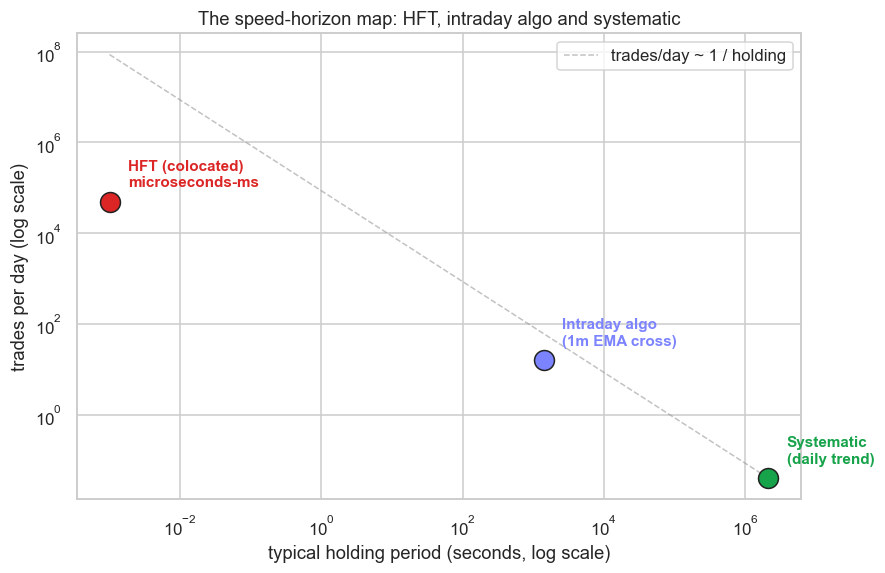
The points fall along a clean diagonal: HFT at roughly 1 millisecond holds and 50,000 trades a day, the intraday algo at about 23 minutes and 16 trades a day, and the systematic book at about 25 days and 0.04 trades a day. They sit at opposite ends of the same axis. The further down and to the right you travel - longer holds, fewer trades - the less infrastructure and capital you need, and the more your edge comes from being thoughtful rather than fast.
That down-right corner is your home. You will not out-engineer a colocated firm and you do not need to: their advantage evaporates the instant your horizon stretches past a few seconds. Choose the horizon where research, not wiring, decides the winner.
When you size up any new strategy idea, ask first: what is its holding period? If the honest answer is seconds, drop it - you are racing people you cannot beat. If it is days, you are on home ground, and the rest of this course is built for exactly that game.
Recap and what is next
- Algorithmic means computer-decided; systematic means rule-based rather than discretionary; HFT is a narrow, speed-defined subset. Three different questions, not three points on a line.
- The tiers differ in latency, holding period, trade frequency, infrastructure, edge source and capital, all at once.
- Real NIFTY data: minute bars move about 1.4 bps with 375 chances a day; daily bars move about 0.50% once a day, the daily move roughly 23 times larger by the square-root-of-time rule.
- HFT (about 1 ms, 50,000 trades a day) needs colocation and crores; systematic (about 25 days, 0.04 trades a day) needs a laptop and patience; intraday algo sits between and is the most cost-sensitive.
- Retail quants belong in the long-horizon corner, where research beats speed.
We have placed the three tiers on the map. The next chapter zooms into the very top of it - the world of microseconds, direct market access and colocation - and proves, with your own measured latency numbers, why that race is physically unwinnable, and why that is genuinely good news for you.