Algorithmic Trading Foundations

A trading idea in your head is worth nothing until it runs without you. The leap from I think a fast moving average crossing a slow one means go long to a process that watches the market, decides, sizes the trade, fires the order, and checks itself - hundreds of times, unattended, without doing something reckless at 2:47 in the afternoon - is the leap this whole module is about. Module D is execution and technology: how a decision actually becomes a fill. We begin at the foundation, the shape that every automated strategy shares no matter how slow or how fast, from a once-a-day rebalance to a microsecond market maker: the algo loop.

The algo loop: data, signal, sizing, order, risk

Strip any trading bot down to its skeleton and you find the same five stages, running in a circle. Market data comes in - a bar, a quote, a depth update. A signal turns that data into an opinion: long, short, or flat. Sizing turns the opinion into a quantity, scaled to your risk budget rather than your conviction. The order carries that quantity to the exchange. And a risk layer sits across the whole thing, clipping size, blocking trades that breach a limit, and able to halt everything. Then the next bar arrives and the loop turns again.

The single most important discipline in bot design is to keep these stages separate. The signal should not know how big your account is. The sizing should not know which broker you use. The risk gate should be the last word, independent of how clever the signal feels. When you braid them together - sizing logic buried inside the signal, risk checks sprinkled through the order code - you get a system nobody can reason about, and reasoning about it is the only thing standing between you and a runaway loss.

Event-driven versus polling

There are two ways to make the loop turn, and the choice colours your whole architecture. Polling means you ask on a timer: every second, every minute, you pull the latest quote or the latest bar and run the loop once. It is simple, easy to reason about, and perfectly adequate for strategies whose edge lives on the scale of minutes or days. Its weakness is latency and waste - you might poll a hundred times and find nothing changed, or miss a sharp move that happened between two polls.

Event-driven means the market pushes to you: a websocket streams every tick or depth change, and each message triggers one turn of the loop. You react the instant something happens, which is the only way to compete where microseconds matter. The cost is complexity - you now handle out-of-order messages, reconnections, buffering, and bursts. Most retail and systematic strategies are happily polling; the higher you climb toward high-frequency work, the more the world becomes event-driven, and Chapter 32 goes deep on the feeds that drive it.

State and idempotency

A naive loop computes a signal and sends an order. A correct loop remembers what it has already done. The bot is a state machine: at any moment it is flat, long, or short, and the only thing that should move it between states is a genuine change in the signal. This is why our first example does not blast an order on every bar where the fast average sits above the slow one - it acts only when the desired state actually flips, and skips the bar otherwise.

That skip is idempotency: applying the same instruction twice must have the same effect as applying it once. Networks retry. Processes crash and restart mid-session. A websocket can deliver the same tick twice. If "go long" naively appends a buy each time it is seen, a restart that replays the morning will leave you triple-long by lunch. The defence is to make every decision relative to current state, not to fire blind. Watch the loop step through ninety recent one-minute bars of RELIANCE:

# The algo loop on real 1m bars: data -> signal -> sizing -> order intent -> risk. No orders sent.
import os
from datetime import datetime, timedelta

import numpy as np
from openalgo import api, ta

client = api(
    api_key=os.getenv("OPENALGO_API_KEY", "your_api_key_here"),
    host=os.getenv("OPENALGO_HOST", "http://127.0.0.1:5000"),
)

# --- DATA: recent 1m bars for one liquid name ---
end = datetime.now().strftime("%Y-%m-%d")
start = (datetime.now() - timedelta(days=6)).strftime("%Y-%m-%d")
df = client.history(symbol="RELIANCE", exchange="NSE", interval="1m",
                    start_date=start, end_date=end)
close = df["close"].values
stamps = df.index

# --- SIGNAL: 9/21 EMA crossover, computed once, vectorised ---
fast = np.asarray(ta.ema(df["close"], 9))
slow = np.asarray(ta.ema(df["close"], 21))
up = ta.crossover(fast, slow)     # fast crosses above slow -> go long
dn = ta.crossunder(fast, slow)    # fast crosses below slow -> go flat

BUDGET, MAX_QTY = 100_000, 60     # sizing budget and a hard position cap (risk)
position, held, n_signals, blocked = 0, 0, 0, 0
print("time      price    fast    slow  signal  ->  intent       qty")

# --- LOOP: walk the most recent bars as if they arrived one by one ---
for i in range(len(close) - 90, len(close)):
    if not (up[i] or dn[i]):
        continue
    target = 1 if up[i] else 0                 # desired state from the signal
    if target == position:                     # IDEMPOTENCY: already there, skip
        continue
    price = close[i]
    if target == 1:                            # SIZING on entry
        want = int(BUDGET // price)
        qty = min(want, MAX_QTY)               # RISK gate: clip to position cap
        blocked += qty < want
        intent, held = "BUY (enter)", qty
    else:                                       # exit flattens whatever we hold
        qty, intent, held = held, "SELL (exit)", 0
    print(f"{stamps[i]:%H:%M}  {price:7.1f}  {fast[i]:6.1f}  {slow[i]:6.1f}    "
          f"{'up' if up[i] else 'dn'}   ->  {intent:11s} {qty:3d}")
    position, n_signals = target, n_signals + 1

print(f"\n{n_signals} signals in the last 90 bars; {blocked} risk-capped; final state: "
      f"{'LONG' if position else 'FLAT'}. (sandbox-safe, no orders placed)")

time      price    fast    slow  signal  ->  intent       qty
14:08   1321.8  1321.6  1321.6    up   ->  BUY (enter)  60
14:13   1319.3  1321.2  1321.4    dn   ->  SELL (exit)  60
14:37   1319.9  1319.7  1319.7    up   ->  BUY (enter)  60
14:38   1319.1  1319.6  1319.7    dn   ->  SELL (exit)  60
14:53   1319.7  1318.5  1318.4    up   ->  BUY (enter)  60
15:15   1318.3  1319.2  1319.2    dn   ->  SELL (exit)  60

6 signals in the last 90 bars; 3 risk-capped; final state: FLAT. (sandbox-safe, no orders placed)

Six state changes fired across those ninety bars, three of them sized at the position cap rather than the raw budget quantity, and the bot finished the window flat. Notice the risk gate doing its quiet job: the budget wanted more shares than the cap allowed, so the order was clipped to 60 every time. The signal proposes; risk disposes. And notice the rapid in-and-out - a long at 14:08 reversed five minutes later, another reversed in a single bar. That churn is not a bug in the code; it is the honest behaviour of a raw crossover on noisy intraday data, and it is exactly the kind of cost-bleeding whipsaw a real execution layer has to tame.

OpenAlgo as the order gateway

The fourth stage - the order - is where your tidy Python meets the messy outside world. You do not want strategy code speaking a different dialect for every broker, juggling auth tokens and symbol formats and rate limits. That job belongs to an order gateway: a single, normalised interface that takes a clean instruction like buy 60 RELIANCE NSE at market and handles the translation, the credentials, and the plumbing to whichever broker sits behind it.

This is the role OpenAlgo plays. Your signal and sizing logic call one consistent Python and REST interface; OpenAlgo carries the order onward and hands back order IDs and fills you can reconcile. It also offers an analyzer mode - sandbox trading - that runs the identical code path and validates every order without sending a single real one to the exchange. The same five-stage loop you just watched can run in sandbox first, prove that its state machine and risk gate behave, and only then be pointed at a live account by flipping a setting, not by rewriting the bot.

What the bot sees

The print loop shows the decisions; a picture shows the world that produced them. Here is one full session of RELIANCE one-minute bars with the two moving averages and every crossover marked, so you can see precisely what the bot reacted to:

Copy

# What the bot sees: a 9/21 EMA crossover firing on a recent RELIANCE intraday series.
import os
from datetime import datetime, timedelta
from pathlib import Path

import matplotlib

matplotlib.use("Agg")
import matplotlib.pyplot as plt
import numpy as np
import seaborn as sns
from openalgo import api, ta

client = api(
    api_key=os.getenv("OPENALGO_API_KEY", "your_api_key_here"),
    host=os.getenv("OPENALGO_HOST", "http://127.0.0.1:5000"),
)

end = datetime.now().strftime("%Y-%m-%d")
start = (datetime.now() - timedelta(days=6)).strftime("%Y-%m-%d")
df = client.history(symbol="RELIANCE", exchange="NSE", interval="1m",
                    start_date=start, end_date=end).tail(375)   # ~one session
close = df["close"]
fast, slow = ta.ema(close, 9), ta.ema(close, 21)
up = ta.crossover(fast, slow)
dn = ta.crossunder(fast, slow)
t = np.arange(len(close))

sns.set_theme(style="whitegrid")
fig, ax = plt.subplots(figsize=(11, 5))
ax.plot(t, close.values, color="#3a3a3a", lw=1.1, label="RELIANCE 1m")
ax.plot(t, fast, color="#7c83ff", lw=1.3, label="EMA 9")
ax.plot(t, slow, color="#16a34a", lw=1.3, label="EMA 21")
ax.scatter(t[up], close.values[up], marker="^", s=90, color="#16a34a", zorder=5, label="buy signal")
ax.scatter(t[dn], close.values[dn], marker="v", s=90, color="#dc2626", zorder=5, label="exit signal")

ax.set_title("Algo loop view - 9/21 EMA crossover signals on RELIANCE 1m", fontsize=13)
ax.set_xlabel("minutes into the window")
ax.set_ylabel("price (Rs)")
ax.legend(loc="best", framealpha=0.9)
fig.tight_layout()
out = Path(__file__).with_suffix(".png")
plt.savefig(out, dpi=110, bbox_inches="tight")
print(f"{len(close)} bars, {int(up.sum())} buy and {int(dn.sum())} exit signals "
      f"({close.index[0]:%d-%b %H:%M} to {close.index[-1]:%d-%b %H:%M}). Saved {out.name}")

Live output

375 bars, 10 buy and 11 exit signals (25-Jun 09:15 to 25-Jun 15:29). Saved 02_signal_chart.png

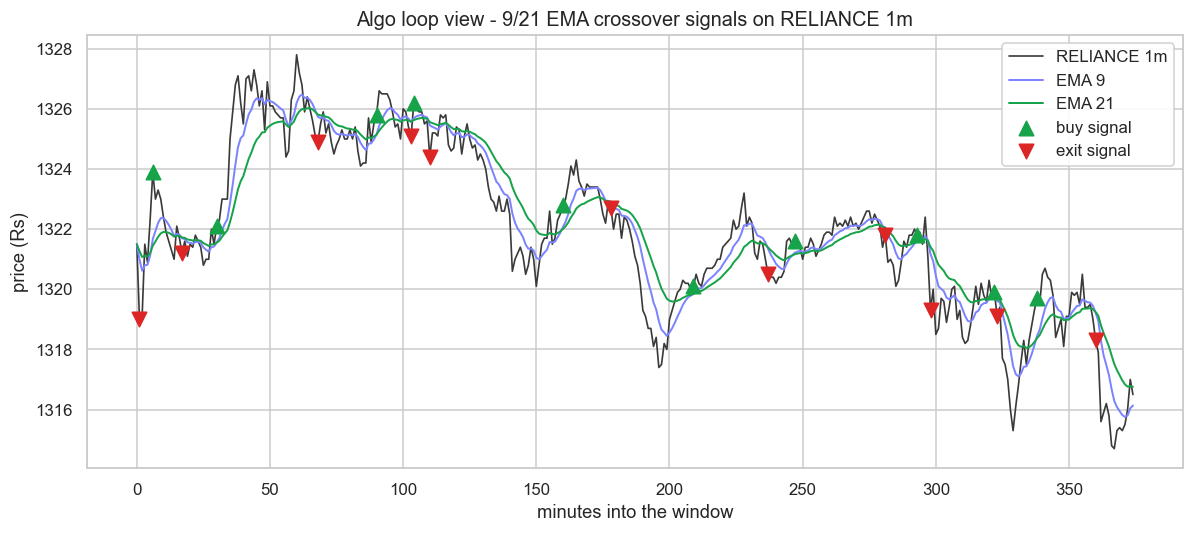
Across a single 375-bar session on 25 June the raw crossover fired ten buy signals and eleven exits - twenty-one round-trip decisions in one day on one symbol. Lay a realistic cost on each of those flips and the strategy is almost certainly underwater before any edge appears. That gap between the clean signal on the chart and the bruising arithmetic of trading it is the entire reason Module D exists. The loop is the easy part; making it survive contact with spreads, latency, queue position and risk limits is the hard part, and it is what separates a backtest from a business.

We now have the universal skeleton. Next we sharpen it: Chapter 30 sets the same loop spinning at three very different speeds - high-frequency, intraday algo, and systematic - and asks the honest question of where a retail quant can actually compete, and where the laws of latency say you simply cannot.