Linear Algebra, Covariance and PCA

A single Nifty stock looks like a line on a chart. Eight of them look like a tangle. But a quant does not see eight tangled lines - a quant sees a cloud of points in eight-dimensional space, and the whole craft of portfolio risk is learning to look at that cloud from the right angle. Linear algebra is the machinery that rotates the cloud until its hidden structure jumps out. When we do that to a basket of Indian large-caps, something striking falls out: most of what looks like eight separate stocks is really one shared force moving them together. That force has a name - the market factor - and in this chapter we extract it with nothing more than a covariance matrix and its eigenvectors.

A portfolio is a vector, a universe is a matrix

Start with the two objects every risk model is built from. A vector is just an ordered list of numbers. Your portfolio weights are a vector: hold 30% RELIANCE, 25% HDFCBANK, 20% INFY and the rest in cash, and that is the vector w = [0.30, 0.25, 0.20, ...]. A single day's returns across the universe is also a vector. Stack many such daily-return vectors on top of each other, one row per trading day and one column per stock, and you have a matrix - the returns matrix R. For eight stocks over a year of trading, R is roughly 334 by 8.

Almost every quantity you care about is a product of these. Your portfolio's return on a given day is the dot product of the weight vector and that day's return vector: multiply element by element and sum. The dot product is the workhorse of quant finance - a weighted basket, a factor exposure, a signal score, are all dot products. Matrix multiplication is just many dot products stacked, which is why a one-line R @ w can price an entire portfolio's daily path at once.

The covariance matrix: risk in one object

A single stock's risk is its variance - the average squared deviation of its returns from their mean, the square of volatility. But a portfolio is not a bag of independent risks. RELIANCE and LT tend to fall together on a bad day, so their risks add up rather than cancel. To capture that, we need covariance: a number that is positive when two stocks move the same way, negative when they move opposite, and near zero when they are unrelated. Divide covariance by the two volatilities and you get the familiar correlation, bounded between minus one and one.

Collect the covariance of every pair into a grid and you have the covariance matrix C. For eight stocks it is 8 by 8: the diagonal holds each stock's own variance, and the off-diagonal entries hold every pairwise covariance. This one object is the beating heart of every classical risk model. Portfolio variance is the compact quadratic form w' C w - sandwich the covariance matrix between your weight vector on both sides and out comes a single number, the variance of the whole book. Mean-variance optimisation, risk parity, the global minimum-variance portfolio, factor risk decomposition - all of them are just different questions asked of C.

Eigenvectors: the natural axes of risk

Here is the pivot. A symmetric matrix like C has a set of special directions called eigenvectors, each with a number attached called an eigenvalue. An eigenvector is a direction in stock-space that the matrix merely stretches without rotating; its eigenvalue is how much it stretches. For a covariance matrix this has a gorgeous meaning: the eigenvectors are the uncorrelated axes of risk, and each eigenvalue is the variance along that axis. The cloud of daily returns is shaped like a stretched, tilted ellipsoid, and the eigenvectors are simply its principal axes - the long axis, then the next-longest perpendicular to it, and so on.

This is exactly Principal Component Analysis (PCA): eigen-decompose the covariance (or correlation) matrix, sort the eigenvalues from largest to smallest, and read off the directions that carry the most variance. The first eigenvector, the first principal component or PC1, is the single direction in which the basket varies the most. The genius of it is compression: instead of eight correlated stocks, you get a handful of independent factors ranked by importance, and usually the top two or three explain the bulk of everything.

Extracting the market factor

Let us actually do it. The next script builds a real returns matrix for eight liquid Nifty names - RELIANCE, HDFCBANK, ICICIBANK, INFY, TCS, SBIN, ITC and LT - forms the covariance matrix, and eigen-decomposes it.

# Returns matrix for 8 Nifty stocks -> covariance matrix -> PC1, the market factor.
import os
from datetime import datetime, timedelta

import numpy as np
import pandas as pd
from openalgo import api

client = api(
    api_key=os.getenv("OPENALGO_API_KEY", "your_api_key_here"),
    host=os.getenv("OPENALGO_HOST", "http://127.0.0.1:5000"),
)

stocks = ["RELIANCE", "HDFCBANK", "ICICIBANK", "INFY", "TCS", "SBIN", "ITC", "LT"]
end = datetime.now().strftime("%Y-%m-%d")
start = (datetime.now() - timedelta(days=500)).strftime("%Y-%m-%d")

# Build the returns matrix: one column per stock, one row per trading day.
cols = {}
for s in stocks:
    px = client.history(symbol=s, exchange="NSE", interval="D",
                        start_date=start, end_date=end)["close"]
    cols[s] = np.log(px / px.shift(1))
R = pd.DataFrame(cols).dropna()
print(f"Returns matrix R: {R.shape[0]} days x {R.shape[1]} stocks")

def show(names, values, nd=2):
    return {n: round(float(v), nd) for n, v in zip(names, values)}

# Covariance matrix (daily), annualised volatility on its diagonal.
cov = R.cov()
vol = np.sqrt(np.diag(cov) * 252) * 100
print("Annualised vol %:", show(stocks, vol, 1))

# Eigen-decompose the covariance matrix. Eigenvalues = variance along each axis.
evals, evecs = np.linalg.eigh(cov.values)
order = np.argsort(evals)[::-1]          # largest first
evals = evals[order]
evecs = evecs[:, order]
share = evals / evals.sum()

pc1 = evecs[:, 0]
if pc1.mean() < 0:                        # orient PC1 so it points "up with the market"
    pc1 = -pc1

print("Variance share per component %:", [round(float(x * 100), 1) for x in share])
print("PC1 loadings (the market factor):", show(stocks, pc1, 2))
print(f"PC1 explains {share[0] * 100:.1f}% of all variance - the single market factor "
      f"these {len(stocks)} stocks share.")

Returns matrix R: 334 days x 8 stocks
Annualised vol %: {'RELIANCE': 21.4, 'HDFCBANK': 19.8, 'ICICIBANK': 19.0, 'INFY': 28.3, 'TCS': 24.3, 'SBIN': 22.4, 'ITC': 19.0, 'LT': 25.2}
Variance share per component %: [41.6, 22.7, 8.3, 7.8, 6.5, 6.3, 3.4, 3.3]
PC1 loadings (the market factor): {'RELIANCE': 0.31, 'HDFCBANK': 0.31, 'ICICIBANK': 0.25, 'INFY': 0.48, 'TCS': 0.42, 'SBIN': 0.31, 'ITC': 0.18, 'LT': 0.45}
PC1 explains 41.6% of all variance - the single market factor these 8 stocks share.

The headline result is the share of total variance carried by PC1. On this basket and window, PC1 explains about 41.6% of all the variance in the eight stocks - a single direction accounting for more than two-fifths of everything. And look at its loadings: every one is positive. RELIANCE, HDFCBANK, INFY, LT, all of them load the same way on PC1. That is the signature of the market factor. When PC1 moves up, the entire basket tends to rise together; when it moves down, they fall together. It is, in essence, a data-derived version of "the market went up today", discovered without ever being told what an index is.

PC2 and the sector tilt

If PC1 is the market, what is PC2? The second component is the largest source of variance left over once the market move is stripped out, and it is forced to be uncorrelated with PC1. Empirically it almost always turns out to be a sector or style tilt. The chart below draws three views at once: the correlation heatmap, the scree plot of variance per component, and the PC1 and PC2 loadings side by side.

Copy

# Correlation heatmap + PCA scree and PC1/PC2 loadings for 8 Nifty stocks.
import os
from datetime import datetime, timedelta
from pathlib import Path

import matplotlib

matplotlib.use("Agg")
import matplotlib.pyplot as plt
import numpy as np
import pandas as pd
import seaborn as sns
from openalgo import api
from sklearn.decomposition import PCA

client = api(
    api_key=os.getenv("OPENALGO_API_KEY", "your_api_key_here"),
    host=os.getenv("OPENALGO_HOST", "http://127.0.0.1:5000"),
)

stocks = ["RELIANCE", "HDFCBANK", "ICICIBANK", "INFY", "TCS", "SBIN", "ITC", "LT"]
end = datetime.now().strftime("%Y-%m-%d")
start = (datetime.now() - timedelta(days=500)).strftime("%Y-%m-%d")

cols = {}
for s in stocks:
    px = client.history(symbol=s, exchange="NSE", interval="D",
                        start_date=start, end_date=end)["close"]
    cols[s] = np.log(px / px.shift(1))
R = pd.DataFrame(cols).dropna()

# PCA on standardised returns so every stock weighs equally.
Z = (R - R.mean()) / R.std()
pca = PCA().fit(Z)
share = pca.explained_variance_ratio_
load = pd.DataFrame(pca.components_[:2].T, index=stocks, columns=["PC1", "PC2"])
if load["PC1"].mean() < 0:
    load = -load

sns.set_theme(style="whitegrid")
fig, ax = plt.subplots(1, 3, figsize=(15, 4.6))

sns.heatmap(R.corr(), annot=True, fmt=".2f", cmap="rocket_r", vmin=0, vmax=1,
            cbar=False, ax=ax[0])
ax[0].set_title("Correlation of daily returns")

ax[1].bar(range(1, len(share) + 1), share * 100, color="#7c83ff")
ax[1].set_title(f"Scree: PC1 = {share[0] * 100:.0f}% of variance")
ax[1].set_xlabel("Principal component")
ax[1].set_ylabel("Variance explained %")

load.plot.bar(ax=ax[2], color=["#16a34a", "#dc2626"], legend=True)
ax[2].axhline(0, color="#555", lw=0.8)
ax[2].set_title("PC1 (market) and PC2 (tilt) loadings")
ax[2].tick_params(axis="x", rotation=45)

fig.suptitle("8 Nifty stocks: correlation, PCA scree and loadings", fontsize=13)
fig.tight_layout()
out = Path(__file__).with_suffix(".png")
plt.savefig(out, dpi=110, bbox_inches="tight")
print(f"{R.shape[0]} days, {R.shape[1]} stocks. PC1 {share[0]*100:.1f}%, "
      f"PC2 {share[1]*100:.1f}%. Mean pairwise corr {R.corr().values[np.triu_indices(8,1)].mean():.2f}. Saved {out.name}")

Live output

334 days, 8 stocks. PC1 40.7%, PC2 18.9%. Mean pairwise corr 0.31. Saved 02_corr_heatmap_scree.png

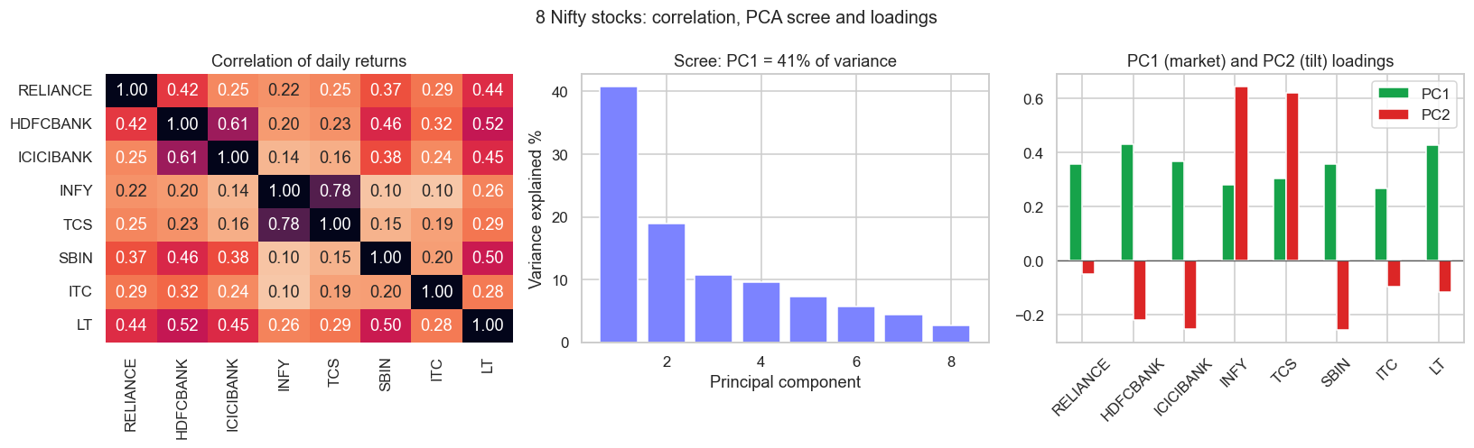
Run it and the structure is unmistakable. The heatmap lights up two tight blocks: INFY with TCS correlate at 0.78 (the IT pair), while HDFCBANK, ICICIBANK, SBIN and LT cluster as the banks-and-cyclicals group. On the standardised (correlation) version, PC1 carries 40.7% of variance and PC2 a further 18.9%, with the average pairwise correlation across the basket sitting at 0.31. And PC2's loadings split the universe cleanly: positive on INFY and TCS, negative on the banks. PC2 is long IT, short banks - a sector spread that PCA found on its own, with no sector labels supplied. The top two components together already explain about 60% of all the joint movement in eight stocks.

These two ideas - that risk lives in a covariance matrix, and that its eigenvectors are the real factors driving a universe - underpin the rest of the quant toolkit. Factor models, statistical arbitrage on the residuals after PC1 is removed, risk-parity allocation, and the principal-component hedges used on options books all start exactly here. Next we close out the mathematics module and turn the covariance matrix into something you can optimise against: building portfolios that trade off return and risk deliberately rather than by accident.