Volatility Modeling (GARCH)

Here is the quant's quiet secret. You cannot forecast tomorrow's return - we proved that. But you can forecast tomorrow's volatility with genuine, useful accuracy, because volatility, unlike returns, has a long memory. Calm begets calm; a storm warns of more storms. The model that captures this - GARCH - is one of the most important tools in all of finance, and it underpins how a quant sizes positions, prices options, and measures risk. If returns are noise, volatility is signal.

Volatility clusters

Recall the stylized facts from Chapter 11: the size of returns comes in runs. A violent day is usually followed by more violent days; a sleepy stretch tends to stay sleepy. Volatility doesn't jump around randomly - it persists. That persistence is exactly the kind of memory a time-series model can exploit, and it's why modelling variance succeeds where modelling returns fails.

EWMA: a first model with memory

The simplest way to capture it is an exponentially-weighted moving average (EWMA) of squared returns: today's volatility estimate is mostly yesterday's estimate, nudged by yesterday's actual move, with older days fading away exponentially. It's the classic RiskMetrics approach - one decay parameter, no fitting required - and it already beats a plain rolling window because it lets recent shocks matter more. GARCH is its smarter, fittable cousin.

ARCH and GARCH in plain words

GARCH builds today's variance from three honest ingredients:

• A baseline (ω) - the long-run average variance the series is pulled toward.
• The ARCH term (α) - how sharply variance reacts to yesterday's shock. A big surprise yesterday raises today's expected volatility.
• The GARCH term (β) - how much yesterday's variance persists into today. This is the memory.

The two weights tell the whole story: α + β measures total persistence. Close to 1 means volatility shocks fade slowly - a spike today still echoes weeks later.

Fitting GARCH to Nifty

Let's fit one and read those numbers off real data:

# Volatility clusters and persists - GARCH(1,1) captures it. Fit one to Nifty.
import os
from datetime import datetime

from arch import arch_model
from openalgo import api

client = api(
    api_key=os.getenv("OPENALGO_API_KEY", "your_api_key_here"),
    host=os.getenv("OPENALGO_HOST", "http://127.0.0.1:5000"),
)

end = datetime.now().strftime("%Y-%m-%d")
r = client.history(symbol="NIFTY", exchange="NSE_INDEX", interval="D",
                   start_date="2021-01-01", end_date=end)["close"].pct_change().dropna() * 100

res = arch_model(r, vol="Garch", p=1, q=1, mean="Constant").fit(disp="off")
alpha, beta = res.params["alpha[1]"], res.params["beta[1]"]

print("GARCH(1,1) fitted to Nifty daily returns:")
print(f"  alpha (reaction to yesterday's shock) : {alpha:.3f}")
print(f"  beta  (persistence of past variance)  : {beta:.3f}")
print(f"  alpha + beta (total persistence)      : {alpha + beta:.3f}   (near 1 = vol clusters strongly)")

next_vol = float(res.forecast(horizon=1).variance.iloc[-1, 0]) ** 0.5
print(f"\nForecast next-day volatility : {next_vol:.2f}%  (annualised ~{next_vol * 252 ** 0.5:.1f}%)")
print("Unlike returns, volatility HAS memory - so it can genuinely be forecast.")

GARCH(1,1) fitted to Nifty daily returns:
  alpha (reaction to yesterday's shock) : 0.103
  beta  (persistence of past variance)  : 0.872
  alpha + beta (total persistence)      : 0.975   (near 1 = vol clusters strongly)

Forecast next-day volatility : 0.83%  (annualised ~13.2%)
Unlike returns, volatility HAS memory - so it can genuinely be forecast.

There's the classic signature: α near 0.10 (a moderate reaction to each day's shock) and β near 0.87 (strong persistence), summing to 0.975 - extremely close to 1. That single number says Nifty's volatility is highly persistent: when the market gets turbulent, it stays turbulent for a long time, and when it calms, it stays calm. And crucially, the model produces a genuine forecast of tomorrow's volatility - something no model could honestly do for tomorrow's return.

Watch it track the storms

Plot the model's estimated volatility over time and you can see it breathe with the market:

Copy

# GARCH's conditional volatility tracks the market's calm and storm.
import os
from datetime import datetime
from pathlib import Path

import matplotlib

matplotlib.use("Agg")
import matplotlib.pyplot as plt
import seaborn as sns
from arch import arch_model
from openalgo import api

client = api(
    api_key=os.getenv("OPENALGO_API_KEY", "your_api_key_here"),
    host=os.getenv("OPENALGO_HOST", "http://127.0.0.1:5000"),
)

end = datetime.now().strftime("%Y-%m-%d")
df = client.history(symbol="NIFTY", exchange="NSE_INDEX", interval="D",
                    start_date="2021-01-01", end_date=end)
r = df["close"].pct_change().dropna() * 100

res = arch_model(r, vol="Garch", p=1, q=1, mean="Constant").fit(disp="off")
ann_vol = res.conditional_volatility * (252 ** 0.5)        # annualised %

sns.set_theme(style="whitegrid")
fig, ax = plt.subplots(figsize=(8, 4.5))
ax.bar(r.index, r.abs() * (252 ** 0.5), color="#c7c9f5", width=2, label="|return| (annualised)")
ax.plot(r.index, ann_vol, color="#dc2626", lw=1.8, label="GARCH volatility")
ax.set_title("NIFTY - GARCH conditional volatility (annualised)")
ax.set_ylabel("Volatility (% annualised)")
ax.legend()

out = Path(__file__).with_suffix(".png")
plt.savefig(out, dpi=110, bbox_inches="tight")
print(f"GARCH vol ranges {ann_vol.min():.0f}%-{ann_vol.max():.0f}% over the period (now {ann_vol.iloc[-1]:.1f}%). Saved {out.name}")

Live output

GARCH vol ranges 9%-37% over the period (now 13.3%). Saved 02_garch_vol.png

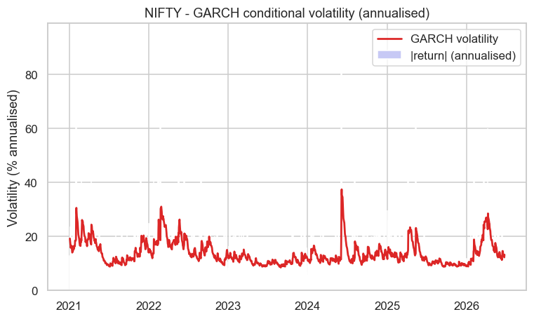
The red GARCH line rises smoothly into every turbulent stretch and sinks back through the quiet ones, riding on top of the jagged daily moves. It isn't reacting to noise day by day; it's tracking the underlying regime of risk - exactly what you want when deciding how much to bet or how to price an option.

Why this is the quant's secret weapon

Forecastable volatility quietly powers a huge amount of real quant work:

• Position sizing. Size down when forecast volatility is high and up when it's low, so each trade carries steady risk (the volatility targeting of Chapter 25).
• Options pricing. Volatility is the single input you can't observe directly - a good forecast is a direct edge in the options market (Module E).
• Risk management. Value-at-Risk and stress models lean on a volatility forecast (Chapter 26).
• Regime detection. A spike in modelled volatility is one of the cleanest signals that the market's character has changed (Chapter 18).

Try it yourself

• Fit GARCH to a single volatile stock and compare its α + β to Nifty's. Is its volatility even more persistent?
• Forecast volatility 10 days ahead instead of 1 (horizon=10). Does the forecast drift back toward the long-run baseline? (It should - that's mean reversion in variance.)
• Compare the GARCH volatility line to India VIX over the same period. How closely does a statistical model of past returns track the market's implied expectation of future vol?

Recap

• Volatility clusters and persists - it has the memory that returns lack, which makes it genuinely forecastable.
• EWMA is a simple, decay-weighted volatility estimate; GARCH is its fittable cousin.
• GARCH(1,1) builds today's variance from a baseline (ω), a reaction to yesterday's shock (α), and persistence of yesterday's variance (β).
• Fitted to Nifty, α + β ≈ 0.975 - volatility is highly persistent, and the model forecasts tomorrow's volatility honestly.
• Forecastable volatility is the engine of position sizing, options pricing, risk management and regime detection - the quant's true edge over the unpredictable.

Volatility was one series with memory. The next is even more tradeable: the relationship between two prices. When two assets are tied together, their spread mean-reverts - and that is the mathematical heart of pairs trading and statistical arbitrage.