Capacity, Turnover and Signal Half-Life

Every retail trader dreams of the strategy that prints money. Few ask the two questions that decide whether it can ever manage real money: how much can it hold, and how long does its edge last? A signal is not just right or wrong - it has a shelf life and a waistline. Push too much capital through it and your own trading eats the edge. Hold it too long and the edge quietly evaporates. This chapter is about those two limits - capacity and half-life - and why they, far more than a backtest Sharpe, decide whether a strategy is a hobby or a business.

Two numbers a backtest never shows you

A backtest reports return, Sharpe and drawdown. It almost never reports the two numbers a fund cares about most. Capacity is the largest amount of capital a strategy can deploy before its own market impact (Chapter 26) drags net returns below the hurdle. Signal half-life is how long the forecast stays useful - the time for its predictive edge, or a mean-reverting mispricing, to decay to half its initial strength. The first limits how big you can be; the second limits how slow you can be. Together they bound the whole economics: capacity times return is the rupees you can earn, and half-life sets how often you must trade to earn them.

The cruel part is that both fight the backtest. A backtest run at one lakh of notional fills at the last traded price and assumes infinite depth, so it sees neither limit. Scale that same idea to a hundred crore and impact appears; trade it live for a year and decay appears. Most "great" strategies are great only at toy size and fresh off the lab bench.

Turnover and the drag of trading

Between capacity and half-life sits turnover - how much of the book you trade per unit time, usually quoted as round trips (a buy and the offsetting sell) per year. Turnover is the bridge, because every trade pays costs: half the spread, brokerage, exchange and regulatory charges, and impact. If a strategy earns a gross edge of g basis points per round trip and trades T times a year, its gross annual return is roughly T times g - but its cost drag is T times (spread plus impact), and that drag scales with turnover just as fast as the edge does.

This is why high turnover is so dangerous. A signal that looks brilliant gross can be a net loser simply because it churns. Doubling turnover doubles both the gross return and the cost, so a strategy survives more trading only if each trade's edge comfortably clears each trade's cost. The honest test is always net of a realistic round-trip cost, never gross.

And turnover is not a free choice - it is set by the signal's half-life. A fast-decaying signal forces you to trade often (high turnover, more cost); a slow signal lets you trade patiently (low turnover, less cost). The half-life you measure directly bounds the turnover you can run, which directly bounds the costs you pay. That is why half-life is the natural place to start.

Signal half-life: the shelf life of an edge

Borrow the idea from physics. A radioactive isotope has a half-life - the time for half of it to decay. A trading signal has the same: the time for its forecasting power, or for a mean-reverting spread, to close half the distance back to fair value. Formally, many signals behave like an Ornstein-Uhlenbeck process (Chapter 44) - a series pulled toward its mean at a measurable speed. Regress the signal's daily change on its lagged level; the slope is the mean-reversion speed, and the half-life is minus the natural log of two divided by that slope. Equivalently, the autocorrelation of the signal decays geometrically, and the half-life is where it crosses one half.

Let's measure it on a real mean-reverting spread - two large private banks tied by the same rate cycle:

# Signal half-life: how fast a mean-reverting spread's edge decays, from autocorrelation.
import os
from datetime import datetime

import numpy as np
import pandas as pd
import statsmodels.api as sm
from openalgo import api

client = api(
    api_key=os.getenv("OPENALGO_API_KEY", "your_api_key_here"),
    host=os.getenv("OPENALGO_HOST", "http://127.0.0.1:5000"),
)

end = datetime.now().strftime("%Y-%m-%d")


def close(symbol):
    return client.history(symbol=symbol, exchange="NSE", interval="D",
                          start_date="2021-01-01", end_date=end)["close"]


# Two large private banks - a mean-reverting spread to measure the half-life of.
df = pd.concat([close("HDFCBANK"), close("KOTAKBANK")], axis=1).dropna()
df.columns = ["HDFCBANK", "KOTAKBANK"]
hedge = sm.OLS(df["HDFCBANK"], sm.add_constant(df["KOTAKBANK"])).fit().params.iloc[1]
spread = df["HDFCBANK"] - hedge * df["KOTAKBANK"]

# Autocorrelation decays geometrically for a mean-reverting series: rho(k) ~ phi**k.
lags = [1, 5, 10, 20, 40]
acf = {k: spread.autocorr(k) for k in lags}

# Ornstein-Uhlenbeck fit: regress the daily CHANGE on the lagged LEVEL.
ds = spread.diff().dropna()
lvl = spread.shift(1).loc[ds.index]
beta = sm.OLS(ds, sm.add_constant(lvl)).fit().params.iloc[1]   # mean-reversion speed (<0)
half_life = -np.log(2) / beta                                  # days to close half the gap

print("Signal half-life from spread autocorrelation decay: HDFCBANK vs KOTAKBANK")
print(f"  hedge ratio (OLS)      : {hedge:.2f}")
print("  autocorrelation decay  : " + "  ".join(f"lag{k}={acf[k]:.3f}" for k in lags))
print(f"  OU mean-reversion beta : {beta:+.4f} per day")
print(f"  HALF-LIFE              : {half_life:.1f} trading days  (~{half_life / 5:.0f} weeks)")
print(f"\nThe edge halves in {half_life:.0f} days, so the signal tolerates only "
      f"~{252 / half_life:.0f} round trips a year before it is just churning costs.")

Signal half-life from spread autocorrelation decay: HDFCBANK vs KOTAKBANK
  hedge ratio (OLS)      : 2.28
  autocorrelation decay  : lag1=0.982  lag5=0.912  lag10=0.839  lag20=0.733  lag40=0.564
  OU mean-reversion beta : -0.0194 per day
  HALF-LIFE              : 35.8 trading days  (~7 weeks)

The edge halves in 36 days, so the signal tolerates only ~7 round trips a year before it is just churning costs.

The HDFCBANK-KOTAKBANK spread (hedge ratio 2.28) has a lag-1 autocorrelation of 0.982, fading smoothly to 0.564 by forty days - the unmistakable geometric decay of a mean-reverter. The fitted half-life is 35.8 trading days, about seven weeks. That single number is enormously practical. It says the spread takes roughly seven weeks to revert halfway, so holding for a few days is pointless and holding for a year is overkill. It says the strategy tolerates only about seven round trips a year - trade faster and you are churning noise and paying costs for the privilege. Half-life turns "how often should I trade this?" from a guess into a measurement.

Half-life is also a decay alarm. Re-estimate it on rolling windows; if a signal that used to revert in seven weeks now takes twenty, or stops reverting at all, the edge is dying (the forecast-decay theme of Chapter 47). Many edges do not vanish overnight - they lengthen and fade, and the half-life is the earliest warning.

Capacity from market impact

Now the size limit. Recall the square-root impact law from Chapter 26: the cost of a trade, in basis points, grows with the square root of your participation - your order divided by average daily volume. Gross alpha, by contrast, does not grow with size at all; an edge of twelve basis points is twelve whether you trade one lakh or one hundred crore. So as you deploy more capital, a fixed edge meets a rising cost, and at some size the cost swallows the edge. That crossover is capacity.

The shape is worth feeling. Net profit in rupees is capital times net edge. At small size the edge is almost untouched but you have little capital, so profit is small. As capital grows, profit rises - more money at a still-healthy edge. But impact keeps climbing as the square root of size, the net edge per trade shrinks, and eventually the shrinking edge overwhelms the growing capital. Net profit peaks, then falls. The peak is capacity.

Copy

# Capacity ceiling: gross alpha is fixed, but square-root impact grows with AUM, so net
# P&L rises, peaks, then falls. The peak is the strategy's capacity.
import os
from datetime import datetime, timedelta
from pathlib import Path

import matplotlib

matplotlib.use("Agg")
import matplotlib.pyplot as plt
import numpy as np
import seaborn as sns
from openalgo import api

client = api(
    api_key=os.getenv("OPENALGO_API_KEY", "your_api_key_here"),
    host=os.getenv("OPENALGO_HOST", "http://127.0.0.1:5000"),
)

SYMBOL = "RELIANCE"
end = datetime.now().strftime("%Y-%m-%d")
start = (datetime.now() - timedelta(days=365)).strftime("%Y-%m-%d")
df = client.history(symbol=SYMBOL, exchange="NSE", interval="D", start_date=start, end_date=end)

adv = df["volume"].tail(20).mean()                 # average daily volume, shares (real)
price = float(df["close"].iloc[-1])                # latest close (real)
sigma_bps = df["close"].pct_change().std() * 1e4   # daily volatility in bps (real)

# Strategy assumptions (the alpha is the modeller's; the impact is calibrated on real data).
GROSS_BPS = 12.0          # gross edge per round trip, before impact
TRADES_YR = 120           # round trips per year (holding ~2 days)
Y = 0.5                   # square-root impact prefactor (see Chapter 26)

aum = np.linspace(1e6, 3e8, 600)                    # Rs 10 lakh to Rs 30 crore
part = (aum / price) / adv                          # participation: order / ADV per trade
impact_bps = 2 * Y * sigma_bps * np.sqrt(part)      # round-trip impact (enter and exit)
net_bps = GROSS_BPS - impact_bps
net_pnl = aum * TRADES_YR * net_bps / 1e4           # net rupees per year

i = int(np.argmax(net_pnl))
cap_aum, cap_pnl = aum[i], net_pnl[i]               # capacity = AUM that maximises net P&L
aum_cr, net_cr = aum / 1e7, net_pnl / 1e7

sns.set_theme(style="whitegrid")
fig, ax = plt.subplots(figsize=(8, 4.5))
ax.plot(aum_cr, net_cr, color="#7c83ff", lw=2.4)
ax.fill_between(aum_cr, 0, net_cr, where=(net_pnl > 0), color="#16a34a", alpha=0.18)
ax.fill_between(aum_cr, 0, net_cr, where=(net_pnl <= 0), color="#dc2626", alpha=0.18)
ax.axhline(0, color="#555", lw=1)
ax.axvline(cap_aum / 1e7, color="#dc2626", ls=":", lw=1.6)
ax.scatter([cap_aum / 1e7], [cap_pnl / 1e7], color="#16a34a", zorder=5)
ax.annotate(f"capacity = Rs {cap_aum / 1e7:.0f} cr\npeak net P&L Rs {cap_pnl / 1e7:.2f} cr/yr",
            xy=(cap_aum / 1e7, cap_pnl / 1e7), xytext=(cap_aum / 1e7 + 5.5, cap_pnl / 1e7 * 0.45),
            fontsize=9, arrowprops=dict(arrowstyle="->", color="#16a34a"))
ax.set_title(f"{SYMBOL} capacity: {GROSS_BPS:.0f} bps gross edge eroded by square-root impact")
ax.set_xlabel("Capital deployed (Rs crore)")
ax.set_ylabel("Net P&L (Rs crore / year)")

out = Path(__file__).with_suffix(".png")
plt.savefig(out, dpi=110, bbox_inches="tight")
print(f"ADV {adv / 1e6:.1f}M sh, sigma {sigma_bps:.0f} bps/day. Capacity ~ Rs {cap_aum / 1e7:.0f} cr "
      f"({part[i] * 100:.2f}% of ADV/trade), where impact has eaten {impact_bps[i]:.1f} of the "
      f"{GROSS_BPS:.0f} bps gross edge; peak net P&L ~ Rs {cap_pnl / 1e7:.2f} cr/yr. Saved {out.name}")

Live output

ADV 18.2M sh, sigma 131 bps/day. Capacity ~ Rs 9 cr (0.37% of ADV/trade), where impact has eaten 8.0 of the 12 bps gross edge; peak net P&L ~ Rs 0.43 cr/yr. Saved 02_capacity_ceiling.png

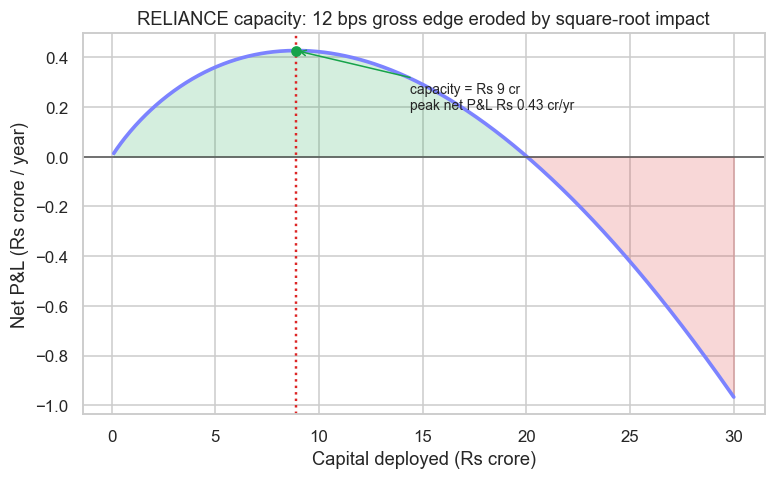
Calibrated on real RELIANCE liquidity - a 20-day ADV of 18.2 million shares and a daily volatility of 131 basis points - a single-name strategy with a 12 bps gross edge traded 120 times a year peaks at a capacity of about nine crore rupees. At that point each trade is just 0.37% of ADV, yet impact has already eaten 8 of the 12 gross basis points, leaving a third of the edge. Peak net profit is a modest Rs 0.43 crore a year, and beyond roughly twenty crore the strategy loses money - more capital makes less. That is a sobering, honest figure: a respectable single-name edge caps out at single-digit crores.

There is a clean punchline buried in the chart. Capacity sits where impact has consumed exactly two thirds of the gross edge, leaving one third. Push past it and you are paying the market more than your idea is worth.

Crowding, decay and sizing to capacity

Two forces make the picture worse over time. Crowding is the first: when other quants discover the same signal, their trading pushes the price the way yours wants to go before you arrive, so your gross edge shrinks and your effective impact rises. A crowded trade can see its half-life collapse and its capacity evaporate together - the August 2007 quant deleveraging was exactly this, dozens of funds holding the same factor and all selling at once. The second force is plain alpha decay: as a pattern is arbitraged away, the edge fades regardless of your size.

The practical response is to size to capacity, not to ambition. Three habits matter:

• Estimate capacity first. Before scaling, compute the AUM where impact eats your edge, and run well inside it. Many quants cap a strategy at a fraction of its theoretical capacity to leave room for crowding and bad days.
• Buy breadth, not depth. One name caps at nine crore; thirty uncorrelated names of similar capacity hold thirty times the money at the same per-name impact. Capacity scales with the number of independent bets, which is why diversified, market-neutral books (Module G) manage real size where a single pair never could.
• Re-measure constantly. Half-life and capacity are not constants. Track them live; when half-life lengthens or net edge thins, cut size or retire the signal before it bleeds.

That closes Module E. We have learned to model what mean-reverts, to forecast and to know when a forecast is dying, and now to size and pace a strategy to its true limits. Module F leaves the world of pure time series for the richest instrument set in Indian markets - futures and options - where carry, the Greeks and volatility itself become the things we trade.