Module H · Backtesting, ML & Portfolio Construction - Chapter 71

Feature Engineering, Labeling and Leakage

The part of ML that decides everything - building point-in-time features, labeling with the triple barrier, and stamping out leakage.

NSE

What you'll learn

·Point-in-time features
·Stationary feature transforms
·Fixed-horizon labels
·The triple-barrier method
·Meta-labeling
·Leakage audits

In the last chapter we watched a powerful model score 100 percent in training and 49 percent out of sample, and concluded that in markets, model power is mostly a liability. But there is an even more basic reason most ML strategies die, one that has nothing to do with the algorithm at all: the features and the labels were wrong before the model ever saw them. Garbage in, confident garbage out. This chapter is about the unglamorous craft that quietly decides whether a model has any chance - building inputs that are honestly point-in-time and stationary, attaching labels that reflect how a trade actually plays out, and auditing relentlessly for leakage. Get this right and a simple model can earn its keep. Get it wrong and the fanciest network just memorises your mistakes.

Features must be point-in-time and stationary

A feature is any number you feed the model to describe the state of the market at a decision moment. Two properties separate a usable feature from a trap.

The first is point-in-time correctness: the feature may only use information that was genuinely available at the timestamp it is attached to. This sounds obvious and is violated constantly. A daily close is not known at 9:15 a.m.; a quarterly earnings number is not known until it is released, not on the period it describes; an index constituent list as it exists today quietly excludes the companies that were delisted, which is survivorship bias. The cardinal mechanical fix is alignment: if a feature is computed from a bar, you must shift it so the model at bar t only ever sees values formed at t or earlier. A single missing shift is look-ahead bias (Chapter 67) wearing a data-science hat.

The second property is stationarity. Raw price is non-stationary - it wanders, trends, and never revisits the same level with the same meaning. A model trained on RELIANCE at Rs 900 learns nothing transferable about RELIANCE at Rs 1,300. So we transform prices into quantities whose distribution is roughly stable over time: returns and log-returns, rolling volatility, oscillators like RSI that live in a fixed 0 to 100 range, spreads, ratios, and z-scores. Where you need memory of the level but still want stationarity, fractional differencing keeps just enough of the price series to be predictive while passing a stationarity test. The rule of thumb: never feed a model a raw price level when a return or a normalised ratio carries the same signal without the drift.

Tip

Build every feature as a column, then shift the whole frame by one bar before joining the label. If shifting by one bar destroys your edge, the edge was look-ahead, not alpha.

Labels: the part everyone gets lazy about

If features are the question, the label is the answer you train the model to predict, and it deserves at least as much care. The default everyone reaches for is fixed-horizon labeling: label each event by the sign of the return over the next k bars - up is 1, down is 0. It is simple, and it is quietly broken in two ways. It ignores the path: a trade that sinks 5 percent before crawling back to close 1 percent up is labelled a win, even though any real position would have been stopped out days earlier. And it uses one fixed threshold regardless of regime, so the same 1 percent move is treated identically in a sleepy market and a panicked one. You end up teaching the model outcomes that no tradable rule could ever capture.

The triple-barrier method

The fix, popularised by Marcos Lopez de Prado, is the triple-barrier method, and it is the single most useful labelling idea in quant ML. For each event you set three barriers and label by whichever is touched first:

an upper barrier (the profit-take), placed above entry,
a lower barrier (the stop), placed below entry,
a vertical barrier (the time limit), a fixed number of bars into the future.

If price touches the upper barrier first, the label is +1. If it hits the lower barrier first, the label is -1. If neither is touched before the clock runs out, the vertical barrier gives a 0 (or the sign of the small return there). Crucially, the horizontal barriers are not fixed percentages - they are scaled by each event's own volatility, so a calm day gets tight barriers and a wild day gets wide ones. The label now encodes exactly what a real, risk-managed trade would have experienced: take profit, get stopped, or time out.

The triple-barrier method: whichever barrier the path reaches first sets the label.

Let us build it for real. The example below pulls daily RELIANCE history, constructs three honest point-in-time features (yesterday's return, a 20 day rolling volatility from openalgo.ta, and a 14 period RSI), then labels every bar with volatility-scaled barriers at two times the daily volatility and a 10 bar time limit:

EX 1Point-in-time features and triple-barrier labels on RELIANCENSEch71/01_triple_barrier_labels.py

# Point-in-time features + triple-barrier labels on a real stock, with the label distribution.
import os
from datetime import datetime

import numpy as np
import pandas as pd
from openalgo import api, ta

client = api(
    api_key=os.getenv("OPENALGO_API_KEY", "your_api_key_here"),
    host=os.getenv("OPENALGO_HOST", "http://127.0.0.1:5000"),
)

end = datetime.now().strftime("%Y-%m-%d")
df = client.history(symbol="RELIANCE", exchange="NSE", interval="D",
                    start_date="2021-01-01", end_date=end)
c, h, l = df["close"], df["high"], df["low"]
ret = c.pct_change()

# Point-in-time features: each value is known at that bar's close, never uses the future.
feat = pd.DataFrame(index=df.index)
feat["ret1"] = ret                                  # today's realised return
feat["vol20"] = ta.stdev(ret.fillna(0.0), 20)       # rolling daily volatility (stationary)
feat["rsi14"] = ta.rsi(c, 14)                        # momentum oscillator

# Triple-barrier labelling: barriers scaled by each event's own volatility.
PT, SL, H = 2.0, 2.0, 10                             # profit-take, stop (x daily vol), horizon bars
cv, hv, lv, vv = c.values, h.values, l.values, feat["vol20"].values
labels = np.full(len(c), np.nan)
for i in range(len(c)):
    vol = vv[i]
    if np.isnan(vol) or vol == 0.0 or i + H >= len(c):
        continue
    up, dn = cv[i] * (1 + PT * vol), cv[i] * (1 - SL * vol)
    out = 0                                          # time barrier unless a level is touched
    for j in range(i + 1, i + H + 1):
        if hv[j] >= up:
            out = 1; break                           # profit-take hit first
        if lv[j] <= dn:
            out = -1; break                          # stop hit first
    labels[i] = out

lab = pd.Series(labels, index=df.index, name="label").dropna()
names = {1: "profit-take (+1)", -1: "stop (-1)", 0: "time barrier (0)"}
dist = lab.value_counts()
total = len(lab)

print(f"RELIANCE NSE daily  events={total}  PT={PT}xvol  SL={SL}xvol  horizon={H} bars")
for k in (1, -1, 0):
    n = int(dist.get(k, 0))
    print(f"  {names[k]:<18}: {n:4d}  ({100*n/total:4.1f}%)")
print(f"  features used      : {', '.join(feat.columns)}")
up_share = 100 * int(dist.get(1, 0)) / total
print(f"SUMMARY: {total} vol-scaled events, {up_share:.1f}% resolved at the profit-take barrier first.")

Live output

RELIANCE NSE daily  events=1329  PT=2.0xvol  SL=2.0xvol  horizon=10 bars
  profit-take (+1)  :  640  (48.2%)
  stop (-1)         :  567  (42.7%)
  time barrier (0)  :  122  ( 9.2%)
  features used      : ret1, vol20, rsi14
SUMMARY: 1329 vol-scaled events, 48.2% resolved at the profit-take barrier first.

Across 1,329 events, the labels split 48.2 percent profit-take, 42.7 percent stop, and 9.2 percent time barrier. That is a healthy, near-balanced target - far better than the lopsided mush a naive up-or-down label produces, and every label corresponds to an outcome a real position would have lived through. The slight tilt toward profit-takes reflects the gentle upward drift of the stock over the window, not a tradable edge by itself.

To see what a label actually means, the next example marks the outcome of a few sample events directly on the price path - the upper barrier touched (a profit-take), the lower barrier touched (a stop), and the time barrier reached with neither side hit:

Triple-barrier outcomes drawn on the price path chart — EX 2Triple-barrier outcomes drawn on the price pathNSEch71/02_triple_barrier_chart.py

Key idea

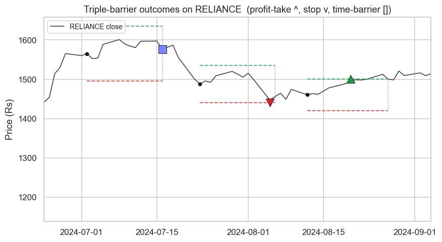
Fixed-horizon labels ignore the path and the regime. The triple-barrier method labels each event by which volatility-scaled barrier - profit-take, stop, or time - is touched first, so the target reflects a real risk-managed trade rather than an untradable snapshot return.

Meta-labeling: a better job for the model

Triple-barrier labels unlock the most successful pattern for ML in trading: meta-labeling. Instead of asking a model to predict direction from scratch (which Chapter 70 showed it cannot do), you let a simple, economically grounded rule decide the side of each trade - a moving-average cross, a mean-reversion trigger, whatever you already trust. You then run the triple-barrier method on just those signalled events and turn the outcome into a binary label: did this particular signal reach its profit-take (1) or not (0)? A secondary model learns to predict that probability and is used purely to filter and size - skip the low-conviction signals, lean into the high-conviction ones. The primary model controls direction; the meta-model controls participation. This division of labour plays to ML's genuine strength, separating good setups from marginal ones, while keeping it away from the question it always fails, calling raw direction.

Note

Triple-barrier outcomes are the natural training target for a meta-model. The +1 versus everything-else split becomes a clean binary label, and the model's predicted probability maps directly to position size.

Leakage audits

Even with point-in-time features and honest labels, leakage - any future information seeping into training - can still inflate a backtest into fantasy. It hides in places the model can never warn you about, so you audit for it deliberately. Three offenders dominate.

First, overlapping labels. A 10 bar triple-barrier label at day t and another at day t+1 share nine days of future price, so consecutive samples are not independent. Train naively and the model effectively sees the same outcome many times and grows falsely confident. The fix is sample uniqueness weighting (down-weight overlapping samples) and purged cross-validation (Chapter 67), which removes samples whose label windows straddle the train and test boundary.

Second, preprocessing leakage. If you scale features or select them using statistics computed over the whole dataset - including the test rows - you have leaked the future into the past. Fit every scaler and feature selector on the training fold only, then apply it to the test fold, every time.

Third, target leakage: a feature accidentally built from the label's own future window, or from a vendor field that gets silently restated after the fact. If a feature looks too predictive, assume it is leaking until you have proven otherwise.

Heads up

Leakage does not announce itself - it shows up only as a backtest that looks too good and live trading that does not match. If your out-of-sample numbers are suspiciously strong, hunt for leaked future information before you believe a single one of them.

Features and labels are where ML in markets is genuinely won or lost, long before any model is fitted. With a stationary, point-in-time feature set and triple-barrier labels you finally have an honest training problem - and several uncorrelated signals begging to be combined into one risk-controlled book. That assembly, from many signals to a single sized portfolio with real risk limits, is the subject of the next chapter.