Cross-Sectional Momentum

Momentum is the workhorse of systematic equity. The idea is almost embarrassingly simple: stocks that have outrun their peers over the last several months tend to keep leading for a while longer, and the laggards tend to keep lagging. Unlike the pairs trade, momentum takes a directional view - but a disciplined, cross-sectional one. It never asks "will this stock go up?" It asks "which stocks are best relative to their peers right now?" - rank the whole universe, buy the top, short the bottom. This chapter builds that long-short machine on the NSE universe, and - true to our honesty rule - lets the Indian data say something uncomfortable about when momentum actually works.

Cross-sectional versus time-series momentum

Two momentums share a name and are easy to confuse. Time-series momentum (also called absolute or trend momentum) looks at one asset's own past - "is Nifty itself trending up over the last six months? If so, hold it; if not, stand aside." Cross-sectional momentum (relative momentum) compares assets to each other - "which stocks have the strongest return relative to the rest of the universe?" The time-series version can swing from fully long to fully in cash depending on the market's own direction. The cross-sectional version is market-neutral by construction: it goes long the leaders and short the laggards, so the broad market's level cancels out and only the spread between winners and losers matters. This chapter is about the cross-sectional kind; pure trend-following on a single series belongs to the time-series world.

Formation and holding periods

Every momentum signal runs on two clocks. The formation period (or lookback) is the window over which you measure past performance. The classic academic choice is the trailing 12 months skipping the most recent month - the "12-1" signal - where you drop the last month deliberately, because over very short horizons stocks tend to reverse rather than continue, and including that noise would poison the signal. The holding period is how long you keep the resulting portfolio before re-ranking and rebalancing, commonly one month.

Horizon is everything here. The same prices behave differently at different time scales: over days to a few weeks markets tend to reverse (overreactions snap back); over 3 to 12 months they tend to trend (true momentum); over 3 to 5 years they revert again (the long-horizon value effect). Pick the wrong clock and the same prices hand you the opposite signal. Our test below uses a 6-month formation and a 1-month hold - a reasonable, widely-used setting that sits squarely in the intermediate-trend zone.

Ranking the NSE universe and building the long-short

Here is the machine. Take a universe of liquid NSE stocks. Every month, rank them by their trailing 6-month return, buy the top third, short the bottom third, hold for a month, then re-rank and rebalance:

# Cross-sectional momentum: each month, go long the winners and short the losers.
import os
from datetime import datetime

import numpy as np
import pandas as pd
from openalgo import api

client = api(
    api_key=os.getenv("OPENALGO_API_KEY", "your_api_key_here"),
    host=os.getenv("OPENALGO_HOST", "http://127.0.0.1:5000"),
)

end = datetime.now().strftime("%Y-%m-%d")
universe = ["RELIANCE", "INFY", "HDFCBANK", "ITC", "TATASTEEL", "ADANIENT", "SBIN",
            "BHARTIARTL", "MARUTI", "SUNPHARMA", "TITAN", "HINDALCO", "AXISBANK",
            "LT", "WIPRO", "POWERGRID"]

prices = pd.DataFrame({s: client.history(symbol=s, exchange="NSE", interval="D",
                                         start_date="2021-01-01", end_date=end)["close"]
                       for s in universe})

monthly = prices.resample("ME").last()
momentum = monthly.pct_change(6)            # 6-month return = the ranking signal
forward = monthly.pct_change().shift(-1)    # next month's return = the test

ls = []
for date in momentum.index:
    score = momentum.loc[date].dropna()
    if len(score) < 6:
        continue
    n = len(score) // 3
    winners, losers = score.nlargest(n).index, score.nsmallest(n).index
    ls.append(forward.loc[date, winners].mean() - forward.loc[date, losers].mean())

ls = pd.Series(ls).dropna()
print(f"Cross-sectional momentum (long winners, short losers), monthly rebalance:")
print(f"  Avg monthly long-short return : {ls.mean() * 100:+.2f}%")
print(f"  Win rate (positive months)    : {(ls > 0).mean() * 100:.0f}%")
print(f"  Annualised Sharpe             : {ls.mean() / ls.std() * np.sqrt(12):+.2f}")
print("\nSign and strength depend on the regime - momentum and reversal trade places over time.")

Cross-sectional momentum (long winners, short losers), monthly rebalance:
  Avg monthly long-short return : -0.94%
  Win rate (positive months)    : 47%
  Annualised Sharpe             : -0.67

Sign and strength depend on the regime - momentum and reversal trade places over time.

The honest result

And here is where the data refuses to flatter us. The momentum long-short produced a negative return and a Sharpe of −0.67 over this window. Sort the stocks into groups and the pattern is the opposite of what momentum predicts:

Copy

# Sort stocks into groups by momentum, then check each group's next-month return.
import os
from datetime import datetime
from pathlib import Path

import matplotlib

matplotlib.use("Agg")
import matplotlib.pyplot as plt
import numpy as np
import pandas as pd
import seaborn as sns
from openalgo import api

client = api(
    api_key=os.getenv("OPENALGO_API_KEY", "your_api_key_here"),
    host=os.getenv("OPENALGO_HOST", "http://127.0.0.1:5000"),
)

end = datetime.now().strftime("%Y-%m-%d")
universe = ["RELIANCE", "INFY", "HDFCBANK", "ITC", "TATASTEEL", "ADANIENT", "SBIN",
            "BHARTIARTL", "MARUTI", "SUNPHARMA", "TITAN", "HINDALCO", "AXISBANK",
            "LT", "WIPRO", "POWERGRID"]

prices = pd.DataFrame({s: client.history(symbol=s, exchange="NSE", interval="D",
                                         start_date="2021-01-01", end_date=end)["close"]
                       for s in universe})
monthly = prices.resample("ME").last()
momentum = monthly.pct_change(6)
forward = monthly.pct_change().shift(-1)

GROUPS = 4
bucket_ret = {g: [] for g in range(GROUPS)}
for date in momentum.index:
    score = momentum.loc[date].dropna()
    if len(score) < GROUPS:
        continue
    ranks = score.rank()
    labels = pd.qcut(ranks, GROUPS, labels=False)
    for g in range(GROUPS):
        names = labels[labels == g].index
        bucket_ret[g].append(forward.loc[date, names].mean())

avg = [np.nanmean(bucket_ret[g]) * 100 for g in range(GROUPS)]
names = ["Q1\n(losers)", "Q2", "Q3", "Q4\n(winners)"]

sns.set_theme(style="whitegrid")
fig, ax = plt.subplots(figsize=(8, 4.5))
sns.barplot(x=names, y=avg, hue=names, legend=False, palette="viridis", ax=ax)
ax.axhline(0, color="#555", lw=1)
ax.set_title("Next-month return by momentum group (monotonic rise = momentum works)")
ax.set_ylabel("Avg next-month return (%)")
out = Path(__file__).with_suffix(".png")
plt.savefig(out, dpi=110, bbox_inches="tight")
print(f"Group returns (low->high momentum): {[round(float(a), 2) for a in avg]}. Saved {out.name}")

Live output

Group returns (low->high momentum): [1.49, 1.84, 0.91, 0.7]. Saved 02_quintile_returns.png

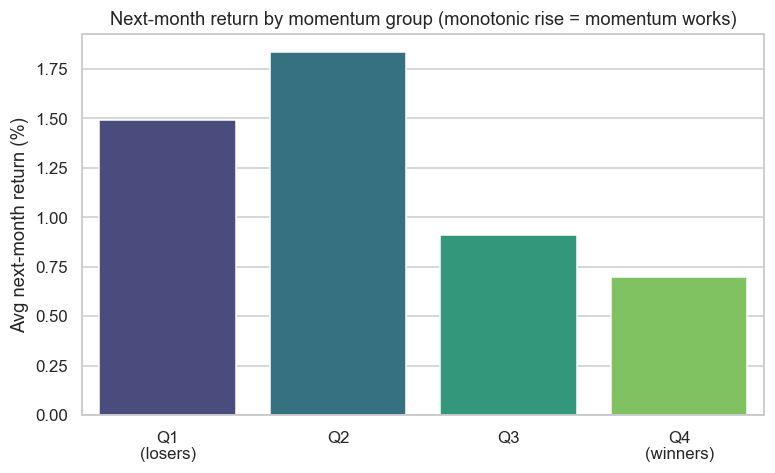
The group returns run roughly downhill, not uphill - the recent losers outperformed the recent winners. In this period and this universe, the Indian market showed short-term reversal, not momentum. We are not going to hide that behind a cherry-picked window. The method is exactly right and is what you are learning; the sign of the edge depended entirely on the regime - precisely the lesson of Chapters 13 and 59. The professional builds the signal at the horizon where the effect is documented and robust, then re-tests it relentlessly across windows rather than trusting one backtest.

Momentum crashes

Even where momentum works on average, it carries a distinctive tail risk that every quant must respect: the momentum crash. Because the short book holds the recent losers - typically beaten-down, high-beta names - momentum suffers its worst, fastest losses precisely when the market rebounds violently after a steep fall. In a sharp recovery the trashed names you are short rocket up hardest, while the winners you are long lag, so the strategy can give back years of slow gains in a few brutal weeks. This pattern showed up across global momentum books in the 2009 recovery and again in the V-shaped rebound of 2020. The returns are negatively skewed: lots of small, steady wins punctuated by rare, severe drawdowns. That asymmetry is why serious momentum desks scale exposure down when volatility spikes and the market is deeply oversold, rather than running the raw signal blind.

Costs and turnover

The other quiet killer is turnover. Re-ranking monthly means a large fraction of the book churns at every rebalance as names cross between the top and bottom thirds. Each rotation pays the spread, exchange charges and securities transaction tax, plus market impact on the less-liquid names - and momentum, by design, chases stocks that have already moved a long way, which are often the ones most expensive to trade. A gross-positive spread routinely turns net-zero or negative once these frictions are honestly subtracted, exactly the warning from the alpha-research chapter (ch59).

The short leg adds an India-specific friction. You cannot hold a delivery short in cash equities overnight here - naked shorting is barred and intraday shorts must be squared off the same day - so a monthly-held short book has to be run through stock futures or the securities lending and borrowing (SLB) market. Futures exist for only the subset of names in the F&O segment, and SLB carries a borrow cost and patchy availability. So a textbook "long-short on the whole NSE universe" is, in practice, long cash plus short futures on the liquid F&O names - a narrower, costlier book than the backtest implies. Model the short side realistically or the strategy is a fantasy.

Beyond momentum

Momentum is just one member of a small family of return drivers. Its natural partner is value - rank by cheapness rather than recent return and buy the unloved names. Value and momentum are famously negatively correlated: value loves the beaten-down stocks momentum is shorting, which is exactly why holding both smooths the ride when one is in a drought. Value, quality, size and low-volatility - the rest of the surviving factor family, and how to combine them into one robust multi-factor book - are the subject of the next chapter (ch61). The single most important lesson momentum teaches is precisely why you need that diversification: no lone factor is dependable, as the −0.67 we just printed makes painfully clear.

Try it yourself

• Flip the signal: go long the losers and short the winners (a reversal strategy). In this window, does the sign flip turn the −0.67 Sharpe positive?
• Change the formation window from 6 months to 12, and add a 1-month skip (the 12-1 signal). Does longer-horizon momentum behave differently from the short version?
• Expand the universe from 16 stocks to a full Nifty-50 list. Does a broader cross-section make the factor steadier (less noise), and how much of the book would actually be shortable via futures?

Recap

• Cross-sectional momentum ranks stocks against each other and trades the spread - long the winners, short the losers - a market-neutral factor bet, distinct from time-series trend on a single asset.
• The signal runs on two clocks: a formation period (lookback, classically 12-1) and a holding period (often a month); short horizons reverse, intermediate horizons trend.
• Honestly, momentum reversed in this Indian window (Sharpe −0.67; group returns ran downhill) - factors are regime- and horizon-dependent, so test across many windows.
• Momentum crashes: the short book detonates in violent recoveries, giving negatively-skewed returns; scale exposure by volatility.
• Turnover and the short leg are costly - monthly churn plus India's no-overnight-cash-short rule force the short side into futures or SLB; model it or the edge is imaginary.

We have built one factor and watched it misbehave. Momentum is real but fragile, and no single factor is enough on its own. The next chapter widens the lens to the rest of the surviving family - value, quality, size and low-volatility - and shows how blending lowly-correlated factors into one multi-factor book is what actually keeps a systematic equity strategy alive when momentum is having a year like this one.